
Objective
Learn about how to use Conditional Formatting based on another cell and other variations around it.
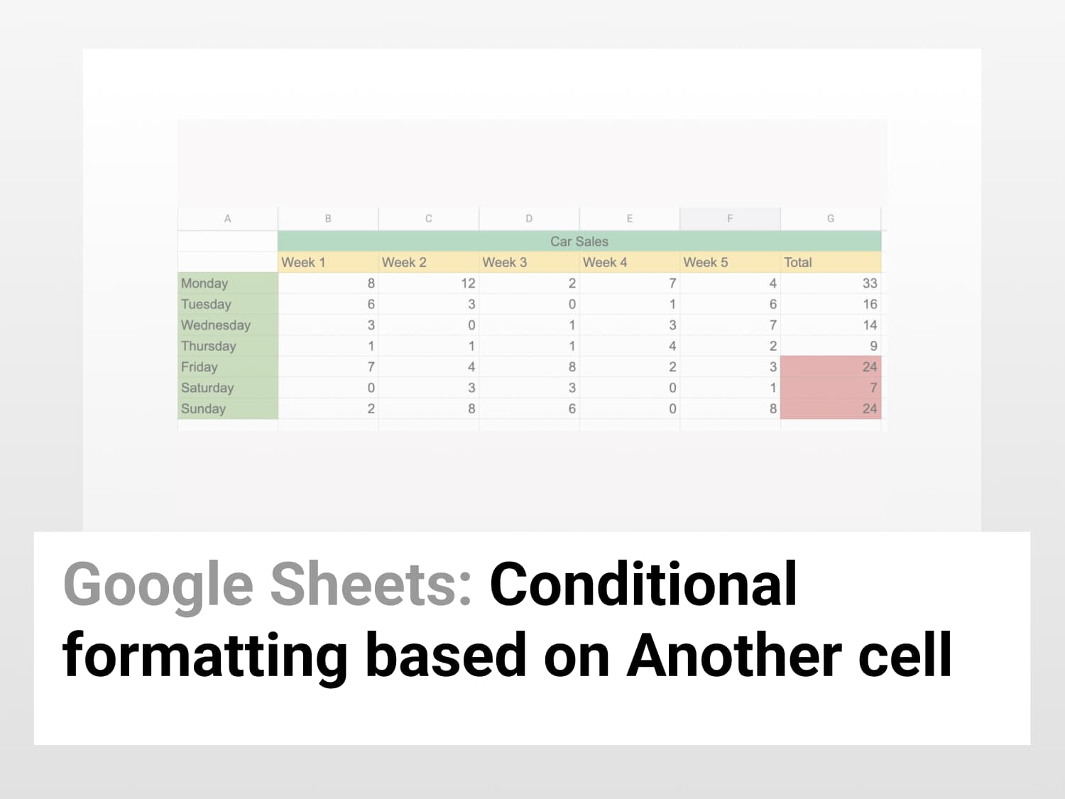
Why use Conditional Formatting based on another cell?
When you’re working with huge tables, all the data can be very overwhelming. Google Sheets provides you with conditional formatting, which helps you visualize data using colours. You can manually add conditions while formatting the data. This helps you in analysing in a better and more efficient way.
Conditional Formatting Based On Another Cell Value Using the Formatting Menu
Step 1: Select the cells you want to highlight
- Open Google Sheets.
- Select the column of cells you want to highlight.

Step 2: Open Conditional Formatting
- Navigate to the Format button in the menu bar. Select Format.
- Click on Conditional Formatting.

Step 3: Modify conditional formatting rules
- Go to the Single Colour tab.
- Also, make sure that the range mentioned in the “Apply to range” tab is the same as the range on which you want to apply conditional formatting.
- Now go to Format Rules and then select Custom formula is.

- In the formula field, enter your custom formula.

- Navigate to Formatting Style and select the colour of your choice.
- Select Done.

Conditional Formatting Based on Multiple Another Cell Values Using the Formatting Menu
Step 1: Select the cells you want to highlight
- Open Google Sheets.
- Select the column of cells you want to highlight.

Step 2: Open Conditional Formatting
- Navigate to the Format button in the menu bar. Select Format.
- Click on Conditional Formatting.

Step 3: Modify conditional formatting rules
- Go to the Single Colour tab.
- Also, make sure that the range mentioned in the “Apply to range” tab is the same as the range on which you want to apply conditional formatting.
- Now go to Format Rules and then select Custom formula is.

- Since you want to apply formatting based on multiple cell values, use the OR function.
- In the formula field, enter your custom formula, as shown below:

- Navigate to Formatting Style and select the colour of your choice.
- Select Done.

See Also
Conditional Formatting in Google Sheets| Quick Guide: Get started with Conditional Formatting in Google Sheets.