In this article, we will have a look at Dynamic Named Range in Google Sheets. We will implement it in a step-by-step fashion on how to create a dynamic range in Google Sheets with a simple example.
What is Named Range?
Named range is a feature in Google Sheets that can be used to give a name to a range of cells. Basically, if we have a range, say B1:B20, which consists of sales records, then we can define this range and give it a name, say SalesRecordRange. If we are to find the sum of these numbers, we can type either =SUM(B1:B20) or simply SUM(SalesRecordRange) to get the sum of the sales data.
What is Dynamic Named Range in Google Sheets?
Dynamic Named Range in Google Sheets is a range which is based on a formula. For example, if we have a shopping list in which we periodically add items to the list along with their prices and a formula that calculates the subtotal. We may add or delete items from the list and we want the subtotal to update accordingly.

This can be achieved using the Dynamic Named Range in Google Sheets. We simply have to declare the shopping list in a dynamic named range, and then use the SUM function to calculate the sum for that range. The Dynamic Named Range would change its value if there is an addition or deletion.
There is no direct way to implement a Dynamic Named Range in Google Sheets.
The dynamic named range is easy to implement in Excel. There is however no direct way to implement Dynamic Named Range in Google Sheets. We can circumvent this limitation by using the INDIRECT function to create a dynamic named range in Google Sheets.
How to implement Dynamic Named Range in Google Sheets
Suppose you have a dataset as shown above in Fig. 1. We want to create a named range in a way such that wherever we add any value to the shopping list, the range gets updated. Below are the steps you can follow to implement Dynamic Named Range in Google Sheets
Step 1. Use the COUNT function to count the number of valid entries dynamically
The COUNT function returns the number of numeric values in a range. We can use this function on the “Price” column to return the number of entries in the shopping list.
Alternatively, we can use COUNTA if you also have string values. If we have any other conditions, we can use the COUNTIF function.

We used the formula =COUNT(B2:B1000)+1 .
The formula COUNT(B2:B1000) returns the number of valid integers between B2 and B1000 (both inclusive). So, if we add another entry, it gets incremented accordingly. B1000 acts as the upper limit here. If your data can have more rows, then you can change this value as per the situation.
Then, we add 1 to the function since we want the index of the last entry to define a named range. The last index will always be one greater than the number of entries since our entries start from 2.
Next, we will have a look at how to implement named ranges in Google Sheets dynamically.
Step 2. Create a reference for the Given Range
In the previous step, we dynamically calculated the position of the last cell. Now we want to reference the range of the sales data. We can do this by using the following formula.
="Sheet1!B2:B"&E3
This returns the dynamic range for the Price attribute in the shopping list. If we enter this formula, it will automatically get converted to the current range.

As you can see in the image above, the formula shows the result “Sheet1!B2:B8” automatically. If we add another entry, it would get updated to Sheet1!B2:B9.
Step 3: Make a Named range for the Shopping List with the dynamic range we just created
- Click on the Formula Cell(In this case E6)
- Go to Data>Named Ranges
- Click “Create New range”
- Give a name to the range. We will be naming our range “TotalPriceRange”
- Click Done

Step 4: Use the INDIRECT function to refer to the dynamic range
Now everything is set up and we just need to calculate the sum. We can do so by using the given formula.
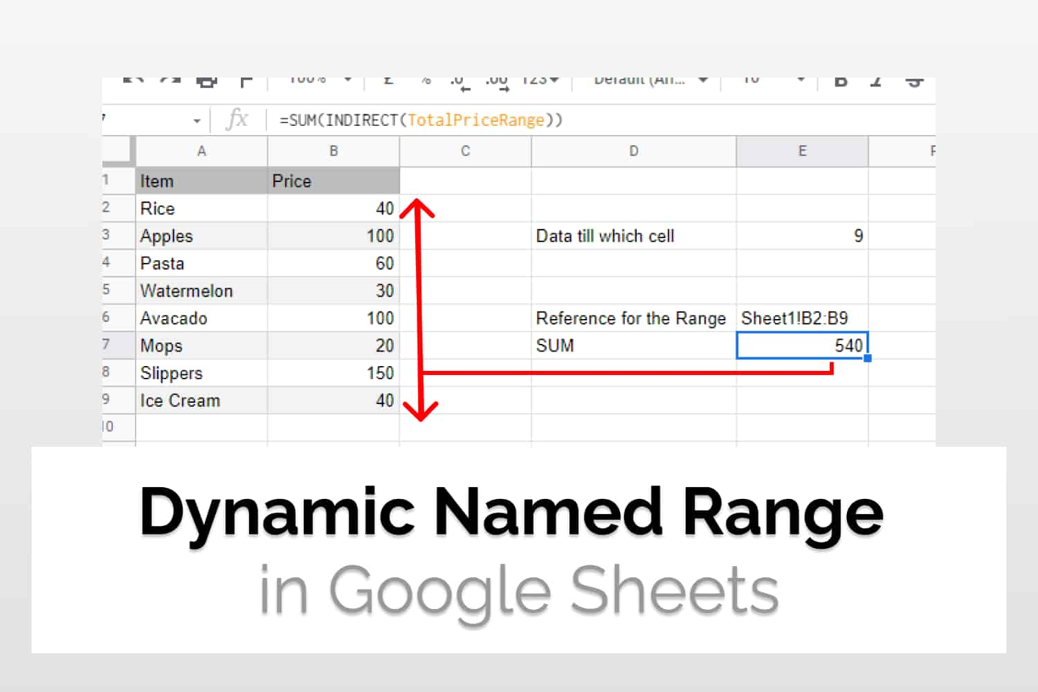
=SUM(INDIRECT(TotalPriceRange))The INDIRECT function basically returns the cell reference specified by a string. Our dynamic range is a string value, if we directly reference it inside the SUM then it won’t work. That is why we need the INDIRECT function to return the reference. The SUM function simply returns the sum over that range.

Let’s add another value to the shopping list.

We added Ice cream to the shopping list and everything automatically got updated. Just keep in mind to either not exceed the limit or keep the limit high enough.
Conclusion
We learned how to implement Dynamic Named Range in Google Sheets using the INDIRECT function. It is ideal for cases where there are additions and deletions to your data frequently. We also saw an example of the same.
See Also
Loved this article on Dynamic Named Range in Google Sheets? Want to know more formulas and functions in Google Sheets? Look at our definitive guide on Google Sheets which covers hundreds of such topics here. Enjoy reading!
Filter Data by Color in Google Sheets: In this article, we would have a look at how to Filter Data by Color in Google Sheets in a simple step-by-step 2 min guide.
How To Calculate Standard Deviation In Google Sheets: We will learn how to calculate standard deviation in Google Sheets using the STDEV function. The STDEV formula is used to find the standard deviation of numbers or a range of values.
How to Calculate Running Balance in Google Sheets: Running balance is a total of transactions already made, or in other words, a cumulative total. In this article, we would have a look at how to implement the same.