The VLOOKUP and the HLOOKUP can be used together to perform 2-dimensional lookup.
Syntax=VLOOKUP(search_key, range, HLOOKUP(search_key, range, index, FALSE), FALSE)search_key – The value to look up for.range – The range of the data to consider to the lookup.index – The row from which to return the value.FALSE – Looks for the exact match. Set to TRUE to search for an approximate match.
//Here, we’re using the HLOOKUP function in place column index in VLOOKUP.
Sample Usage=VLOOKUP(B11, A1:E8, HLOOKUP(B12, A1:E8, 2, FALSE), FALSE)
//The HLOOKUP performs a horizontal search in the range A1:E8 based on the value in cell B12, and then the VLOOKUP returns the corresponding to cell B11.

We will learn how to use Vlookup and Hlookup together in Google Sheets in a combined fashion to refine your searches for a large table.
Background
VLOOKUP and HLOOKUP are two very popular formulas used in Google sheets. They perform vertical and horizontal searches, respectively. Using Vlookup and Hlookup together in Google Sheets can be very powerful. You can combine them to perform 2D searches in a table. It is a very popular practice which a person should know. You can achieve the same using Index Matching as well but anyway, it is a good practice to know about.
Matrix Preparation
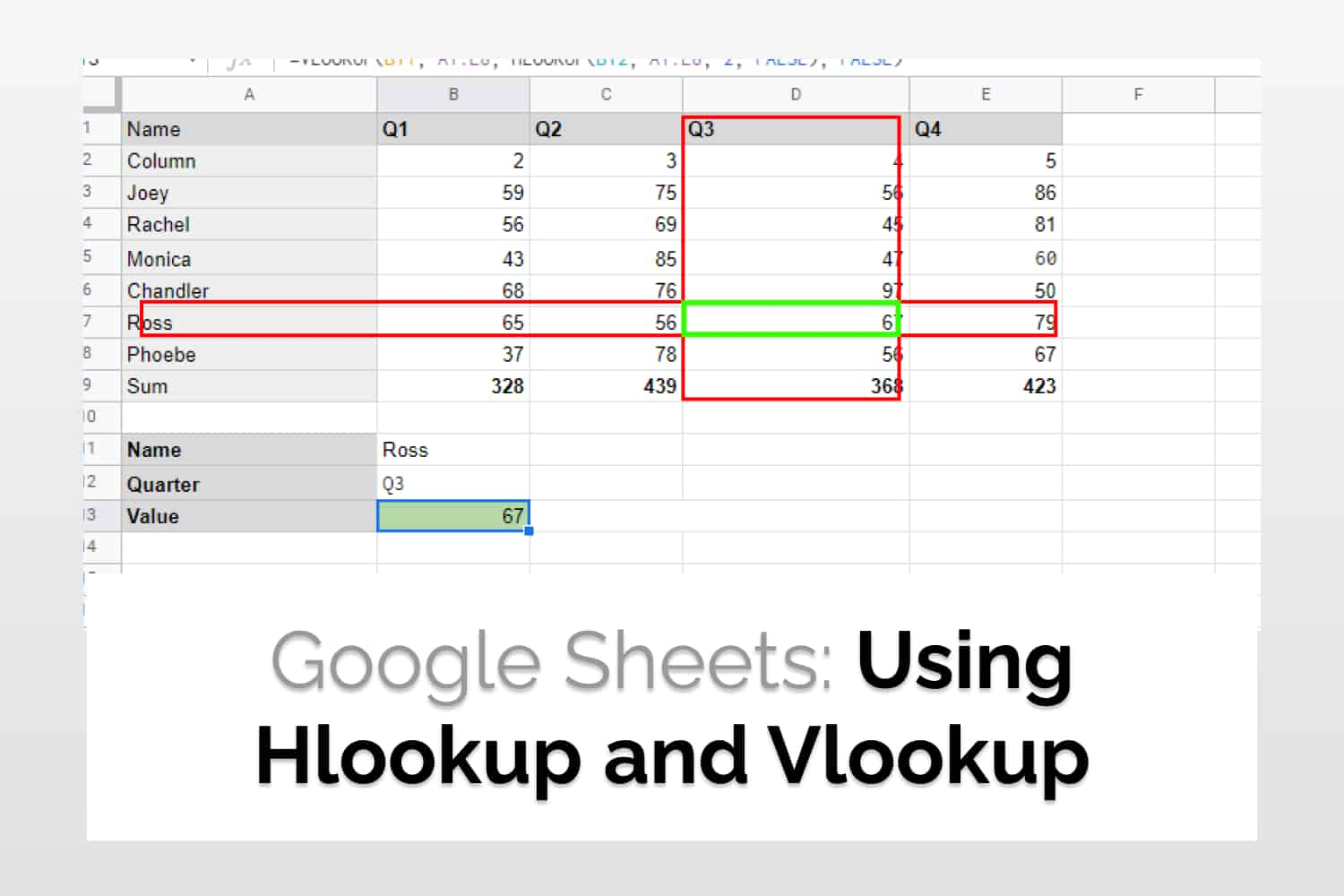
First of all your data needs to have lookup values on both top and left sides. For example, in the following Figure 1, in the given matrix the lookup value on the top consists of the quarter values, and on the left, we have the names of the salesperson. So for example, “Ross” did a sale of 67 units in Q3.

You’ll also need to have an additional row below your first row which will act as an identifier for columns. This is required for the Hlookup-Vlookup combination, so if for some reason you can’t add the additional row, you can consider using Index Matching.
Syntax
Using Vlookup and Hlookup together in Google Sheets is pretty straightforward. But, before getting started, I’ll recommend going through Hlookup and Vlookup so that we already know their functionalities respectively.
Using both of them together is a fairly simple concept, we use the value returned by Hlookup as a row number for VLOOKUP. The syntax for the same is given below.
=VLOOKUP(search_key, range, HLOOKUP(search_key, range, 2, FALSE), FALSE)
Example: Using VLOOKUP and HLOOKUP together in Google Sheets
We come back to the table that we saw earlier.

Suppose we want to find out Ross’s sales in Q3. This table passes the prerequisites for matrix preparation that we talked about earlier. Let’s First make reference cells for us to fetch the arguments for.

The formula that we will write will go in cell B13 and it will fetch the values for search terms from B11 and B12.
Now the formula for the given scenario would be the following.
=VLOOKUP(B11, A1:E8, HLOOKUP(B12, A1:E8, 2, FALSE), FALSE)

As you can see that the value displayed is consistent with the value in the table. Lets see how it was calculated.
HLOOKUP(B12, A1:E8, 2, FALSE) would perform the horizontal lookup and search between the first row values (i.e. Q3). After it successfully finds the value it returns the corresponding column number which, in this case, is 4.

=VLOOKUP(B11, A1:E8, HLOOKUP(B12, A1:E8, 2, FALSE), FALSE) will be calculated next. Since the HLOOKUP section returned 4, this expression was reduced to =VLOOKUP(B11, A1:E8, 4 , FALSE). It will perform a vertical lookup for the value “Ross” and return the correspond 4th column, which in this case is 67.

Conclusion
Hence, using VLOOKUP and HLOOKUP together in Google Sheets we were able to perform searches in a matrix. If you don’t want to add the additional row to your table you can check out Index matching. This article discusses why Index Matching is better than using Hlookup or Vlookup.
See Also
Want to know more formulas and functions in Google Sheets? Look at our definitive guide on Google Sheets which covers hundreds of such topics here. Enjoy reading!
Vlookup in Google Sheets: We will learn about Vlookup in Google Sheets with several examples. We will also learn some advanced Vlookup features.
Google Sheets: Hlookup | Quick Guide: Introduction to Hlookup in Google Sheets