
Highlight Duplicate Cells In Google Sheets
We will have a look at how to highlight duplicate cells in Google Sheets using Conditional Formatting. We will have a look at how to highlight duplicate cells in Google Sheets in both single and multiple columns in Google Sheets.
Need to Highlight Duplicate Cells in Google Sheets
Let’s say you have a list of data of individuals which are indexed by their email addresses. When the data is being handled manually, there is a possibility that your primary key(which is the email in this case) repeats. This can be due to some human error or any logical error. The duplicate entries need to be identified and dealt with, especially if the email is your primary key. You can also check out this article if you want to generate a unique random key for each entry.
Hence in this article, we would look at how to highlight duplicate entries in Google Sheets. You can then choose to either delete the duplicates or handle them however you can.
Duplicate Cells in One Column
We will be using conditional formatting to highlight duplicate cells in a column.
Conditional formatting in Google Sheets allows you to format cells based on some conditions. It is a very handy tool if you are working with color-coding in cells.
- Select the dataset range

- Go to Format->Conditional Formatting. A sidebar will appear which looks like this.

- Cross-check that the range is the same if you want to apply the rule. We now need to add Format rules. Go to Format Rule Dropdown->Custom Formula

- Enter the following Custom Formula =COUNTIF($A$1:$A$50,A1)>1 . Change the range according to your range. This works on the basis of the COUNTIF function. You can read about the COUNTIF function here.
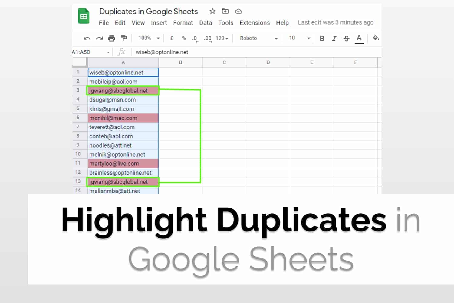
- Select the desired colour and click “Done”. The resultant sheet would look like this.

One advantage of using conditional formatting is that it is dynamic in nature. If you add or edit data in real-time, then, in that case, it would automatically get updated.
Duplicate Cells in Multiple Columns
Suppose all the data that you have is in different columns and you want to find the duplicates. Everything would be the same as before except for two changes.
- Change the Range in “Apply to range” over the entire 2D array. For example, here we will use A1:C50.
- Change the custom formula to suit the entire 2D array. For example, change it to =COUNTIF($A$1:$C$50, A1)>1 for the current example.
The resultant sheet would look something like this.

Conclusion
Hence we looked at a way to highlight duplicate cells in Google Sheets for single or multiple columns using conditional Formatting. You can read more about conditional formatting here. We also used the COUNTIF function to use as a custom formula in Conditional Formatting.
See Also
Want to know more formulas and functions in Google Sheets? Look at our definitive guide on Google Sheets which covers hundreds of such topics here. Enjoy reading!
Conditional Formatting in Google Sheets: Get started with Conditional Formatting in Google Sheets
How to use COUNTIF function in Google Sheets: Learn how to use the COUNTIF function in Google Sheets and its variations.
Delete Empty rows in Google Sheets: In this article, we would see how to delete empty rows in Google Sheets using two different ways.
How to group rows in Google Sheets: We will learn how to group rows in Google Sheets. We will also have a look at nested grouping.