Quick guide
How to create a histogram in Google Sheets:
1. Select the data set to represent as a histogram
2. Go to the Insert tab and select Chart
3. Select Histogram from the Chart type menu
Spreadsheet template with data and chart
- What is a histogram?
- How to create a histogram in Google Sheets
- Customize histogram in Google Sheets
What is a histogram?
A histogram is a graph that groups data points into ranges. These ranges, sometimes referred to as histogram bins or buckets, represent specific intervals which the data values fall into. Histograms are widely used to represent the distribution of numerical data and graphically show the frequency distribution of the data points.
The histogram has a wide range of applications. Any data that needs to be analyzed in terms of distribution over certain ranges would benefit from being plotted as a histogram. Histograms also make analyzing large datasets easier as it enables analysts to observe patterns quickly and derive the essence behind them.
Some popular applications of histograms include:
- In financial trading where it is used in tools like MACD as technical indicators to demonstrate momentum.
- In statistics to represent various demographics and the values that fall into them, eg age groups.
- Histograms are used in signal processing to indicate the distribution of contrast in pixels.
Histograms are essential tools for analysis–and in most cases, they are easy to make. In this tutorial, we will look at how to create histograms in Google Sheets. Google Sheets has the histogram chart built-in, with room for customization as you will see.
How to create a Histogram in Google Sheets
Creating a histogram in Google Sheets can be summarized into 3 simple steps. We need to provide the data, insert a chart, and set up a histogram chart.
Step 1: Provide the data for the histogram in Google Sheets
To create a histogram in Google Sheets we must first begin with the data for the distribution. Below is a table representing investors in a company’s stock and how much profit they made.

The goal of the proceeding steps is to analyze and represent this data in the form of a histogram with the profits grouped into ranges with an indication of their frequency.
Step 2: Open the chart editor
Google Sheets has numerous charts available in its chart menu for visualizing different kinds of datasets.
To insert a chart into a worksheet in Google Sheets, simply do the following:
- Highlight the entire profit column from step 1
- Head over to the Insert menu, then select Chart

- On clicking Chart, the Google Sheet chart dialogue opens. Through this menu, we can select all kinds of inbuilt charts.

Notice that a column chart was selected by default, in the next step we will change this and finalize our histogram.
Step 3: Insert the histogram chart in Google Sheets
To change the selected chart from a column chart to a histogram, follow these steps:
- Click on the drop-down icon in the Chart type box
- Scroll down the list of charts until you find the Histogram chart
- Select this and Google Sheets will render the data in the form of a histogram.

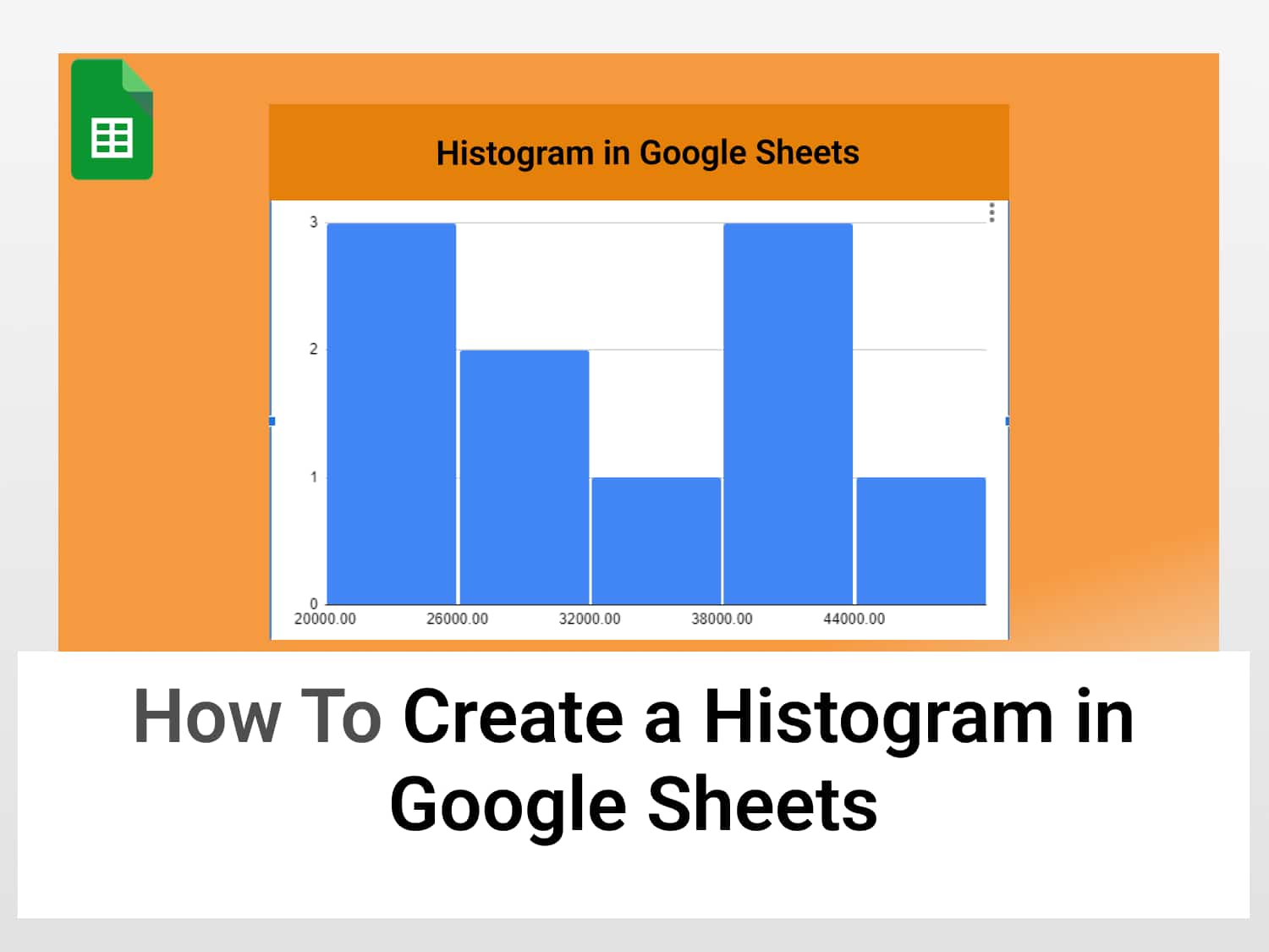
Below is the histogram representing the values from the table. The X-axis represents the histogram bins or buckets, ie, the range of values for the profits. The Y-axis represents the frequencies of the profits.

Customizing the histogram in Google Sheets
There are many customization features available for our histogram in Google Sheets. To view these options you can open the chart editor by clicking on the three dots in the uppermost right corner of the chart.
- On opening the Chart editor you will find two tabs—Setup and Customize.
- The Setup tab is used for certain configuration purposes and modifying how the histogram interprets data.
- The Customize tab contains all the customization features available for the histogram. These are divided into subsections such as Chart style, histogram, Chart and axis titles, etc.
Let us change the color of the histogram
Changing the color of the histogram
To change the color of the histogram simply do the following:
- Open the Chart editor
- Open the Customize tab
- Scroll down to Series and open the drop-down menu
- Select Fill color
- Change the color of the histogram by setting this color to your choice.

Above is our histogram with a new color. We can also change the color of the entire background. To do this we will follow steps similar to those above. The customization option can be found under Chart Style this time from the Customize tab.
- Select Background color
- Pick a color of your choice

Asides from changing colors, there are other ways we can further customize our histogram.
Adding a chart title for the histogram in Google Sheets
If you observe, our chart doesn’t have any title. We can fix this by creating a title in the Customize tab. Let’s follow the steps below to do that :
- Open the Chart editor menu
- Open the Customize tab
- Select Chart & axis title
- Make sure the drop-down menu is currently set to Chart title
- Enter a title for the histogram into the Title text box
- You can also title the horizontal and vertical axis if you like

And that’s it. We have successfully created and customized a histogram in Google Sheets.
Google Sheets makes it easy to create and customize histograms. To do this we simply need to provide a dataset and then insert a histogram from the Chart menu.
Some commonly asked questions
Where is histogram chart in Google Sheets?
The histogram chart is found in the group of charts available by default in Google Sheets. To find the histogram chart in Google Sheets:
- Click on Insert from the tab
- Click on Chart
- A column chart is selected as Chart type by default, so click on the drop-down to open a list of all charts
- Scroll down this list to the category labeled other
- Select the histogram chart
How do I change the number of bins in a histogram in Google Sheets?
To change the number of bins i.e histogram buckets in Google Sheets, simply open the Chart editor, then:
- Go to the Customize tab
- Select Histogram
- Select Bucket Size. This is set to Auto by default but you can pick the new range you want from a list.
See also
Check out some other interesting articles in our blog:
How to create a Bubble Chart in Google Sheets