Syntax=sparkline(data, [options])data refers to the fields you want the Progress Bars for, and options refers to specifying various parameters such as charttype, color, max and min values.
Sample Usage
=SPARKLINE(B2,{“charttype”,”bar”;”max”,1;”min”,0;”color1″,”green”})
//picks value in B3, convert to charttype bar in color green
You can also make a copy of the spreadsheet below to get hands-on experience.
Sample Spreadsheet for practice here
Progress bars in Google Sheets are one of the best ways to keep track of your performance, by looking at the easy-to-interpret charts. Whether you are a student wanting to track your progress while preparing for your exams, or you are a team manager, keeping a track of your team’s progress, learning how to create progress bars can prove to be useful for you.
Google Sheets does not provide a direct way to create progress bars but we found a super-easy way for you to create progress bar charts in Google Sheets with the least amount of effort. By the end of this article, you’ll learn everything about how to create progress charts in Google Sheets using the SPARKLINE Function.
Before that, let’s get a better understanding of the progress bars.
What is a progress bar?
A percentage progress bar is a visual representation of the percentage of progress made in bar graph format. The visualization further aids you with effortless tracking of performance.
Basically, progress bars describe how much percentage of a task has been completed, but visually.

Why a progress bar in Google Sheets?
There is no in-built feature to create progress bars in Google Sheets, it is nevertheless a useful tool. So learning how to create progress bars in Google Sheets can be beneficial.
- To analyze the data in an easy manner
- Helps with quick decision making
This being established that progress bars in Google Sheets are very helpful, let’s move on to the next part now.
How to create a progress bar in Google Sheets
Creating Progress Bars in Google Sheets can be achieved by following a quite straightforward 3-step process.
Here, we use the SPARKLINE Function to create the Progress Bars. The SPARKLINE Function uses the value of the field, along with choice of color to depict the percentage. The function fills the cell with the color with respect to the value of the field selected and the maximum and minimum values for the given data.
Note: The max and min values will be 1 and 0 respectively in the case of percentage.
The syntax of the SPARKLINE function
=SPARKLINE(data, [options])Where, Data refers to the fields you want the progress bars for, and
Options refers to specifying various parameters such as charttype, color, max and min values.
For a better understanding of the SPARKLINE Function, you can also refer to the video link.
Now that we’ve got familiar with the function used to create progress bars in Google Sheets, we can move on to the steps to create them.
Step-by-step guide to create a progress bars in Google Sheets
Step 1: Add the data to Google Sheets
To get started with progress bars in Google Sheets, you’ll firstly need to add the data to the sheet.

Step 2: Add SPARKLINE function syntax to create progress bars
Next, you need to add the following SPARKLINE Function Syntax in the cell C3:
=SPARKLINE(B3,{“charttype”, “bar”; “max”, 1; “min”, 0; “color1”, “purple”})

Next, you need to copy the same or simply drag the tab for the rest of the rows as shown.
The final result of the progress bars in Google Sheets will look like this.

Step 3: Format the progress bars using IF function (Optional)
You can also format the Progress Bars according to your convenience to get an even better idea of the data. This can be done using the IF Function while creating the Progress Bars in Google Sheets. You can modify the Progress Bars in such a way that the Bars are represented in different colors if the value in the field is above/below a particular limit.
For example, look at the Syntax below:
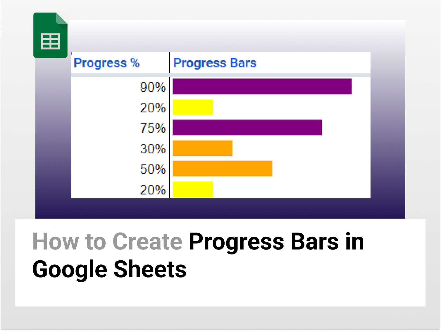
=SPARKLINE(B3,{“charttype”, “bar”; “max”, 1; “min”, 0; “color1”, IF(B3>0.6, “purple”, IF(B3>0.25, “orange”, “yellow”))})
What the IF condition in this formula does is change the color of the progress bar to purple if the task is more than 60% complete, orange if more 25% but less than 60%, and if less than 25% complete then yellow.

Next, drag the formula cell to apply the syntax to all the rows as shown below.
Step 4: View the Progress Bars
The Progress Bars in Google Sheets would finally look like this after adding the IF Function conditions to it.

Conclusion
Keeping a track of your progress towards an objective is a really important and crucial task. Progress bars can help decrease your effort and time by providing you with easily readable visuals.
Hope this article helped you!
See Also
Want to know more formulas and functions in Google Sheets? Look at our definitive guide on Google Sheets which covers hundreds of such topics here. Enjoy reading!
How to Create Funnel Charts in Google Sheets: Learn how to create funnel charts in Google Sheets in 4 easy steps
How to select all Checkbox in Google Sheets: Learn how to create a Select All Checkbox in Google Sheets.
How to Use XLOOKUP Function in Google Sheets: Learn how to use XLOOKUP Function in Google Sheets in 3 different ways.
How to Use the CHOOSE Function in Google Sheets: Learn how to use the CHOOSE Function in Google Sheets in 4 minutes using different examples.