The P-value can be found by using the T.TEST function.
Syntax=T.TEST(array1, array2, tails, type)array1 – The first range of data.array2 – The second range of data.tails – Specifies the type of distribution: 1 – one-tailed distribution, 2- two-tailed distribution.type – An integer value that can be 1 (paired t-test), 2 (2-sample t-test with equal variance), or 3 (2-sample t-test with unequal variance).
Sample Usage=T.TEST(A3:A9, B3:B9, 1, 3)
//This will return the P-value for the data in the ranges A3:A9 and B3:B9 for a one-tailed distribution with unequal variance.
P-value is one of the most important statistics measures for any dataset. It is usually used to determine the correctness of certain hypotheses. And knowing how to find P-value in Google Sheets would be quite useful.
Ever wondered, how can you determine if your data obtained is correlated or not? Are the results obtained worth considering or not?
This is exactly what P-value can help you with. Google Sheets provide you with a very strong tool to find the P-value without actually doing the calculations manually.
By the end of this article, not only will you be able to identify the significance of your results, but also how to find the P-value in Google Sheets.
What is P-value?
The P-value is a statistical measurement used to determine whether a data is statistically significant or not. It basically measures the probability of obtaining the observed data provided the null hypothesis is true.
The null hypothesis being true refers to basically considering that any difference seen in the observed data and the measured data is completely out of chance and that both the data are the same.
Why do we use P-value?
You would have already understood by now, the importance of P-value when dealing with data. Post calculating the P-value, you can easily determine how close you are to your results.
Usually, a significant value is determined as a threshold for calculations, i.e., 0.05 is considered a threshold value. The lower the P-value, the more likely it is for your data to be statistically correlated.
How to find P-value in Google Sheets?
Here is a spreadsheet template for a hands-on experience of the Function.
Free Google Sheets Spreadsheet Template
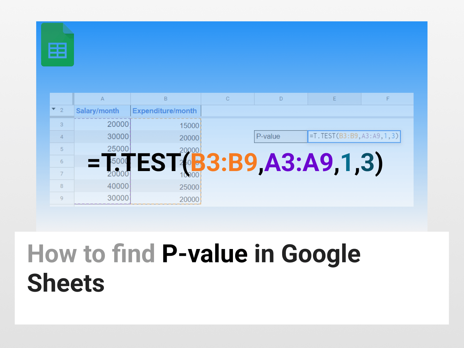
Let’s say, you have this dataset representing the average salary per month and average expenditure per month.

Syntax
=T.TEST(array1,array2,tails,type)
Where, Array 1 refers to the first range of data;
Array 2 refers to the second range of data;
Tails refers to 1- one-tailed distribution, 2- two-tailed distribution;
Type refers to an integer value that can be 1 (paired t-test), 2 (2-sample t-test with equal variance), or 3 (2-sample t-test with unequal variance).
Step 1: Add the Syntax for P-value in Google Sheets
Add the T.TEST Syntax in the cell where you want the P-value to be displayed.

Step 2: Specify the Syntax Parameters
Add the range 1, 2, tails, and type according to the requirements.

Here, we have selected B3:B9 and A3:A9 as range1,2 respectively, and one-tailed distribution and 3 for a 2-sample t-test with unequal variances
Note: Variance can be calculated using VAR Function in Google Sheets.
Final P-value

We obtained a P-value lower than 0.05 showing that our data is statistically significant and thus can be correlated. This is a very simple and straightforward method to calculate P-value in Google Sheets.
Conclusion
Calculating P-value in Google Sheets is a relatively simple task with the help of the T.TEST Function. All you need to do is enter data, specify the type and tails and you will have your answer in no time.
It saves you from all those tedious calculations that need to be done when done manually.
Hope this article helped you!
See Also
Want to know more formulas and functions in Google Sheets? Look at our definitive guide on Google Sheets which covers hundreds of such topics here. Enjoy reading!
How to use Does Not Equal Function in Google Sheets: In this article, you can learn how to use the Does Not Equal Function in Google Sheets.
How to create a Dynamic Named Range in Google Sheets: Learn how to create a Dynamic Named Range in Google Sheets in 4 easy steps. Easy 5-min read guide to help you out find the required hacks to do the task.
How to create a Funnel Chart in Google Sheets: A basic 4-min guide explaining how to create Funnel Charts in Google Sheets.