Quick guide
To hide rows based on cell value in Google Sheets, follow these steps:
Step 1: Select the data range.
Step 2: Create a filter.
Step 3: Specify conditions and apply the filter.
Sample spreadsheet template with formulas here.
- Filtering options in Google Sheets
- Hide rows using the filter menu
- Hide rows based on numbers
- Hide rows based on dates
Sometimes we might be working with data that needs sorting or we simply might need to view only specific portions of a large data set. In such situations, it’s pretty helpful to have a way to automatically create a filter that easily hides rows or columns of interest in our tables or data sets.
Fortunately for us, such a tool does exist. Google Sheets makes a provision for sorting operations through the filter menu.
In this guide, we will learn how to hide rows based on cell values in Google Sheets. We will consider various examples of how to hide rows in Google Sheets based on the texts, numbers, or even references to other data stored in cells. This can be quite handy for various reasons.
Benefits of hiding rows based on cell value in Google Sheets include:
- Quickly sort through data based on our exact preferences.
- Conveniently copy only sorted data to another table if needed.
- Quite handy on extensive datasets as trying to hide data manually would be a very tedious process.
Before we head on to the examples, let’s take a look at how it is possible to hide rows based on cell value in Google Sheets.
The Filter menu in Google Sheets and how it works
To hide rows based on cell values in Google Sheets we use the filter menu. This tool helps us specify conditions that if met will result in our desired outcome — which is usually to return portions of the entire data set.
The filter menu isn’t just for hiding rows or columns based on cell values, it is a powerful tool that enables us to sort data very easily in Google Sheets. You can perform several operations thanks to the wide range of options available, some of them include: cell value, color, text, and other properties that can be used to differentiate cells.
In this tutorial, we’ll be learning how to hide cells based on their values. So, let’s get to it!
How to hide rows based on cell value in Google Sheets using the Filter menu
First, let’s begin by providing the data to filter. The table below contains information about contestants in an online competition that took place across multiple days.

Ordinarily, to sort through the data in this table and return, say, the information of the contestants from the USA only while hiding the rows for those from other countries, the steps would be to:
- Select a particular row by clicking the row number.
- Right-click to open the options menu for that row ➡ Choose hide row.
- Repeat the steps above for each row of interest.
This works just fine. But imagine you had thousands of data rows and wanted to sort based on specific dates. Now you see the limitations.
So let’s look at the convenient Filter menu option that can make hiding cells based on cell value in Google Sheets and other similar processes a breeze.
To use the Filter tool, we will follow three basic steps.
Step 1: Select the entire data range you want to apply a filter to
To filter the data in a data set we need to highlight the entire data. We can select either specific rows or columns too but we will use the entire table in this example because we will be working with multiple fields in the data set.
Step 2: Create a filter in Google Sheets
To create a filter simply do the following with your data still highlighted:
- Click on Data
- Then select Create a filter from the options.

Notice the filter icon that now appears at the top of the various columns in our table. Simply click on this to open the filter options for the data contained in that column.

Step 3: Specify your filter conditions
In the filter menu, you will find several criteria which you can use in creating your desired filters. Categories include filter by cell color, filter by values, filter by condition, etc.
Let’s use the Filter by values option:
- Click on the filter icon in the Candidate column
- Expand the Filter by cell values option
- Select Adam Luoise from the names and then click OK

The row containing the information for Adam Luoise will be hidden from the data set.
There are also other quite handy options in the filter menu, for instance, you can filter by text formats in the given cells — what the texts contain or don’t.

Also, you can enter a direct text value and this will be evaluated as a condition. If we want to see all the contestants from a particular country, e.g. USA, all we need to do is simply type that into the box.

Hide rows based on cell value in Google Sheets — numbers
So far we have considered text values contained in the cells. However, the filter tool also works well with numbers.
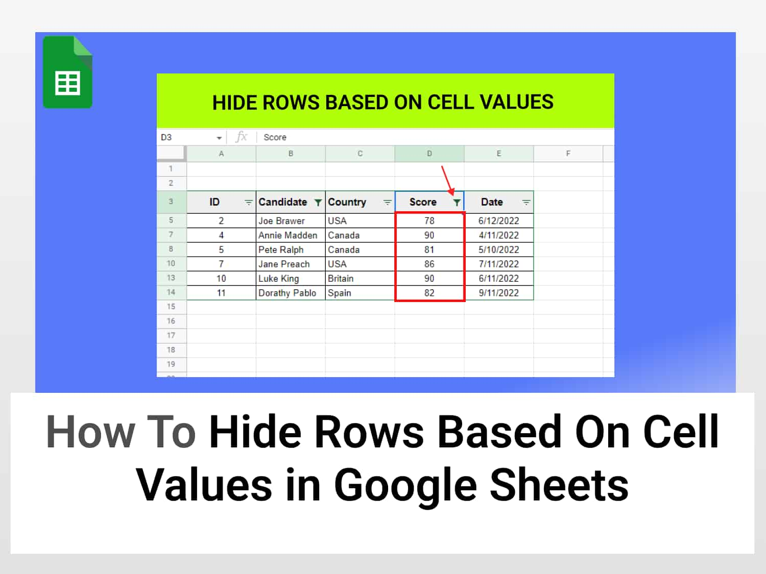
Let us sort the data in our table and return only data for contestants who scored above 70.
- Click on the filter icon in the Score column
- Select filter by condition and set the condition to greater than.
- Enter 70 into the box.

Google Sheets will check every score and only select those cells which contain above 70 as a value.

Rows 1, 6, and 8 do not contain values above 70 and therefore have been hidden.
Hide rows based on cell value in Google Sheets — Dates
Another very common criterion used for filtering data is date value. There are so many reasons you could want to sort your data based on dates, from sales records to subscription services to purchases, the list is endless.
The Filter tool makes it possible to hide rows in Google Sheets based on dates.
- Click on the filter icon in the date column
- Select filter by condition
- Select exact date and enter the desired date

This will return only rows that contain values matching the specified date

The filter menu enables us to hide rows in Google Sheets based on a wide range of properties. We can quickly leverage this feature in making our tasks easy.
Some commonly asked questions
Can you conditionally hide rows in Google sheets?
Yes, you can. Google Sheets’s filter enables you to specify conditions using “greater than” or “less than” and so on, this can hide rows in Google Sheets conditionally.
To hide rows based on condition in Google Sheets: open the filter menu ➡ filter by condition ➡ enter your desired condition.
How to hide/unhide rows in Google Sheets
You can use the filter to hide rows as we have seen in this article. Though there are other options, the filter menu is easy to use and effective for many use cases.
To unhide the rows you filtered out, click on the Data tab with the entire data selected then ➡ Remove filter.
See Also
Check out some other similar articles on our blog:
https://blog.tryamigo.com/copy-and-paste-only-visible-values-in-google-sheets/
Delete empty rows in Google Sheets
https://blog.tryamigo.com/how-to-group-rows-in-google-sheets/