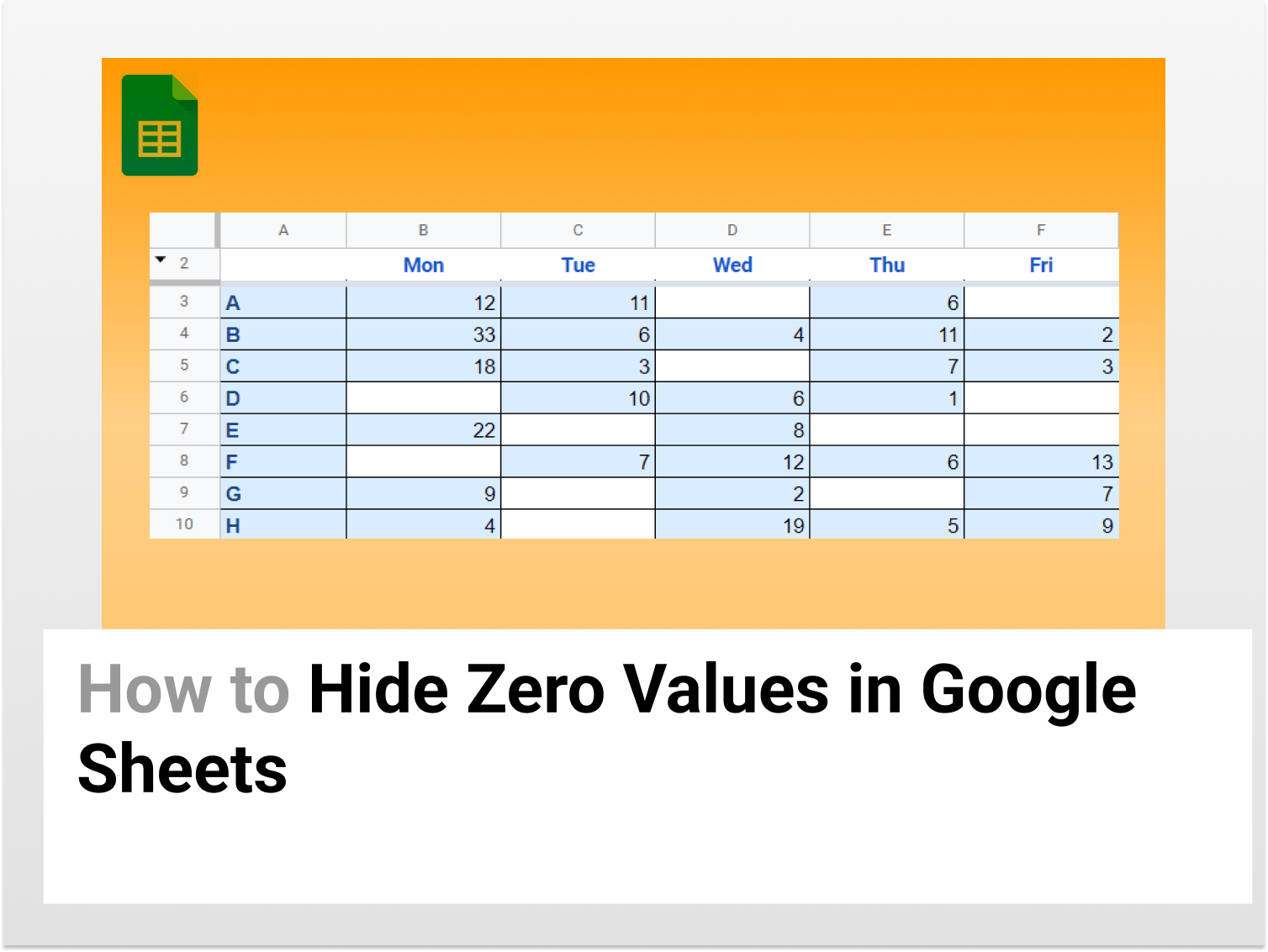
While working with data, we often come across zero values. However, sometimes users might wish to hide/remove those zero values from the data. Unlike Excel, Google Sheets doesn’t have a direct function to do the same. But, there are some ways to hide the zero values in Google Sheets.
This article will help you understand a few easy hacks to hide the zero values in Google Sheets from your data. By the end of this page, you’ll not only know how to hide zero values from your data but also how to remove them completely.
Why hide zero values in Google Sheets
The presence of zero values in the data is important for calculation purposes but looking at a blank cell helps with quicker interpretation than looking at the digit ‘0’. Therefore, it is better to hide those values for better visual representation. Since the values are just hidden, the formulas in Google Sheets would also include zero values unless wished otherwise.
How to hide zero values in Google Sheets
Three different ways are described below to hide zero values in Google Sheets.
You can also make a copy of the spreadsheet below for hands-on practice.
Sample Spreadsheet for Hands-on Experience
Option 1: Hide zero values using Conditional Formatting
Conditional Formatting can be used to hide zero values in Google Sheets.
Step 1: Add Data to Google Sheets
Firstly, add the data to Google Sheets. Here, we have added data for say, student A to H for the weekdays. You can find several cells containing the zero value.

Select the entire dataset, A3:F10 for the formatting.
Step 2: Go to Format Tab > Conditional Formatting
Next, go to the Format Tab and select Conditional Formatting from the list.

A dialog box will now appear on the right side of the screen.
Step 3: Changes in Conditional Formatting Rules Box
Now, all you have to do is go to ‘Format Rules’ box and from the dropdown select ‘is equal to’ followed by adding ‘0’ in the next tab. Next, you need to set the text color and the cell color to white.
‘Is equal to’ => 0
Voila! You can now hide zero values in Google Sheets.
The final view of the spreadsheet would be something like this.

Option 2: Hide zero values using Custom Number Formatting
You can also use the custom number formatting to hide zero values in Google Sheets just by making a few edits in the number format toolbox.
Step 1: Add Data to Google Sheets
Add the data to Google Sheets and select the entire dataset, A3:F10 for the formatting.

Step 2: Go to Format Tab > Number >Custom Number Format
Next, you need to go to the Format Tab and Number and then select the Custom Number Format from the list.

A dialog box will appear on the screen.
Step 3: Edit the Custom Number Format to 0;-0;;@
Now, you need to enter the following format in the Custom Number Format tab.
0;-0;;@
The Custom Format in Google Sheets consists of four parts: Positive, Negative, Zero, Text.
Here, we set
- Positive to ‘0’ to look the same way it is.
- Negative to ‘-0’ to have a negative sign in front of the actual value
- Zero to nothing as we want to hide the values
- Text to @ as this will return the exact same text
Click on Apply and you are done.
All the zero values in the spreadsheet are now hidden.
This is how the final data would look like.

Option 3: Remove Zero values using Find and Replace
Now, if you don’t just want to hide but completely remove the zero values in Google Sheets, you can use the simple-to-use Find and Replace Function.
Step 1: Add Data to Google Sheets
Add the data to Google Sheets and select the entire dataset, A3:F10 for the formatting.

Step 2: Go to Edit Tab > Find and Replace
Next, you need to go to the ‘Edit‘ Tab and click on ‘Find and Replace‘.

A dialog box will appear on your screen.
Step 3: Find ‘0’ and Replace by a blank.
Next, in the Find an Replace dialog box, enter 0 in the ‘Find’ field and leave the ‘Replace’ field blank.
Select the ‘Match case’ and ‘Match entire cell contents’ and click on ‘Replace All’.
And, the zero values are removed from the Google Sheets.

All the cells containing the zero values have now been replaced by a blank space.
Conclusion
Hiding/removing zero values from a dataset can thus be easily achieved using either conditional formatting, custom number formatting or by simply replacing the zero values with a blank space.
Hope this article helped you!
See Also
Want to know more formulas and functions in Google Sheets? Look at our definitive guide on Google Sheets which covers hundreds of such topics here. Enjoy reading!
Conditional Formatting Based On Another Cell in Google Sheets: Learn how to use Conditional Formatting Based On Another Cell in Google Sheets.
Does Not Equal Function in Google Sheets: Learn how to use Does Not Equal in Google Sheets in this 4-min easy guide
How to Create Progress Bars in Google Sheets: Learn how to create Progress Bars in Google Sheets in a straightforward way in a 5-minutes guide.
