FV function: Use to calculate the future value of an investment based on periodic compounding interest rates.
Syntax=FV(rate, number_of_periods, payment_amount,[present_value],[end_or_beginning])rate: the interest rate per period.number_of_periods: the number of periods over which payments are made. So, if you pay over every month, the annual interest rate would be divided by 12.payment_amount: represents the periodic payment amount (i.e., your monthly payment amount)present_value: [Optional – 0 by default] represents the present value of an investment at its beginning date (i.e., how much you invested)end_or_beginning: [Optional – 0 by default] represents the end or the beginning date when making payments. For example, 0 indicates the due amount paid at the end of a period, and 1 means at the beginning.
Sample Usage=FV(0.25%, 12, -10000, 0, 1)
//Returns the future value of an investment of 10,000 for 12 months at an interest rate of 0.25 percent.
The FV function in Google Sheets is used to calculate the future value of an investment based on periodic compounding and interest rates. To calculate the FV value in google sheets, it takes three arguments: a principal, a rate, and a number of periods.
Generally, keeping track of finances is easier with google sheets. And the FV function is just another tool that helps you keep track of your finances. So let’s see how to use FV function in Google Sheets.
You have to take note of some parameters before learning how to calculate your future investment. So, that brings us to the syntax of the FV function:
- Calculate the future value of an investment
- Calculate the value of a lump sum investment
- Calculate a loan payback
How to Calculate Future Value in Google Sheets
Future Value (FV) is the value of a single cash flow or multiple cash flows that occur at a given date in the future. The FV function allows you to calculate the future value of a single cash flow or multiple cash flows occurring at specific dates in the future.
You can also use it to calculate the present value of an investment today, given its future value and interest rate. For example, suppose you invest $10,000 today with an annual interest rate of 5%. Then, the FV function can help you determine how much money will be earned after five years if no withdrawals are made.
This guide shows some examples of how to use the FV function in Google Sheets when calculating the future value of an investment in three different scenarios:
So, let us learn how to use the FV functions to calculate an investment’s future value.
How to use FV function in Google Sheet to calculate the future value of an investment
For Instance, I want to add $10,000 at the beginning of every month for a year. If the annual interest of my account is 3%, then we have all the parameters to calculate the future value of this investment.
Step 1: Enter all the parameters into the sheets as shown in the image below;

Note: The interest rate of 3% is divided by12. The number of payments is 12, which was done over one year. The payment amount is negative as the money is going out. The present value is 0, and the payment time is 1.
Step 2: Input the FV function in Google Sheets to calculate the future value of that investment after one year. And here is how to do it:
= FV (0.25%, 12, -10000, 0, 1)
Step 3: Hit on Enter

So, as you can see, the future value of the investment is $121,662.80.
Here is a copy of a template you can use to calculate the future value using the FV function in Google Sheets for investments like this one.
How to use the FV function in Google Sheets to calculate the value of a lump-sum investment
Another task the FV function in Google Sheets can handle is an investment in a lump sum, a one-time investment. So, if I decide to pay $20,000 in an account for the next ten years over an interest rate of 2%, we can also find out the future value using the FV function in Google Sheets.
Here is a quick guide on how to calculate this.
Step 1: Break down the parameters in the spreadsheet as shown below.
Interest rate; 2%
Payment period;10
Payment amount; 0
Present value; -2000

Step 2: Enter the FV formula as written below.
=FV (2%, 10, 0, 20000, 1)
Step 3: Press enter.

This will return $24,379.89, which is the future value of the investment given the parameters.
How to use FV function in Google Sheets to calculate a loan payback
We can use the FV function in Google Sheets to calculate a loan payback period. It is a great way to determine how long it will take to pay back your loans and how much interest you can expect to pay over that period.
For instance, I need to pay back my loan of $100,000 in one year by paying $8,000 by the end of each month at a 5% interest rate. Here is how to know if you would be able to pay the loan in one year.
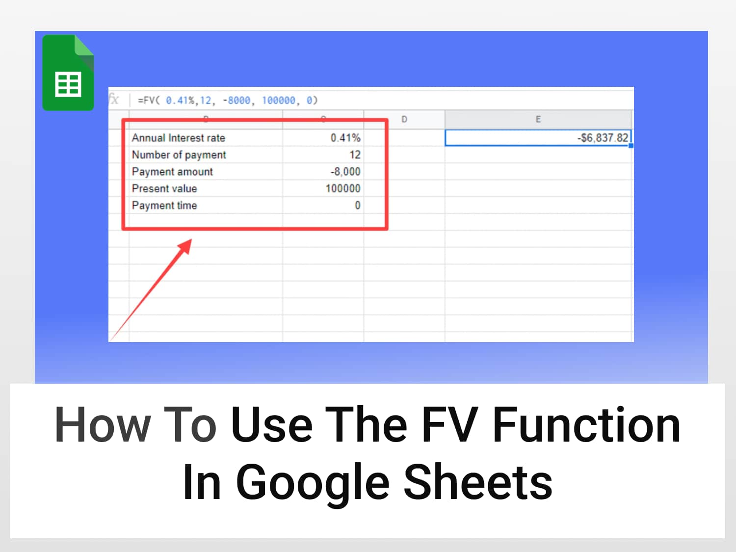
Step 1: Enter the parameters in the spreadsheet.

That makes 12 payments. The present value is $100,000 because we took a loan and have not paid anything. So, while the PV is positive, the payment amount is -$8,000.
Step 2: Input the FV function formula; =FV (0.41%, 12, -$8000, 10000, 0)

Upon pressing Enter, we get -$6,837.82 as the result, showing that I will not be able to pay up the loan over a year with the interest rate and monthly payment.
Conclusion
In this article, we have seen the syntax of the future value formula in Google Sheets and how it can be used to calculate the future value of an investment. We have also seen how to use the FV function in Google Sheets to calculate the value of a lump-sum investment, future investments, or loan payback amount.
See also
You can check out our other related posts for most tutorials on Google Sheets:
https://blog.tryamigo.com/pv-function-in-google-sheets/
https://blog.tryamigo.com/use-coupncd-function-in-google-sheets/
https://blog.tryamigo.com/how-to-calculate-cagr-in-google-sheets/