How to use SUBTOTAL Function in Google Sheets

Reading Time: 6 minutes

What it does – Calculates the subtotal of a range of cells.

Syntax
=SUBTOTAL(function_code, range1, [range2, ...])
function_code – The type of function to use in the subtotal aggregation. See the table below for various codes.

range1 – The range of cells on which to calculate the subtotal.

range2, ... – [Optional] Additional ranges over which to calculate subtotals.

Sample Usage
=SUBTOTAL(9, B3:B7)
//Returns the subtotal for the range B3:B7. The function code 9 is for SUM.

=SUBTOTAL(1, A1:A8, B1:B8)

//Calculates the subtotal of the averages of the ranges A1:A8 and B1:B8.

Table of Contents

What is the SUBTOTAL Function?

The SUBTOTAL function in Google Sheets is a quite versatile function. The SUBTOTAL function can calculate the subtotal of a range of cells. Now, you might wonder why a simple SUM function itself can’t be used to calculate subtotal in Google Sheets. Let’s consider a case where you have hidden or filtered data, the SUM function will not be able to exclude the hidden data which may cause an error in the result and this is exactly where the SUBTOTAL function in Google sheets comes to our rescue.

By the end of this article, you’ll be able to perform various functions using the SUBTOTAL function in Google sheets.

Why do we need a SUBTOTAL Function?

The SUBTOTAL function in Google sheets can be used for the following purposes:

Calculating Subtotals of the lists of data
Calculations excluding the hidden or filtered data rows/columns
Using as a Dynamic Function Selector

Figure 1: Difference between SUM and SUBTOTAL Function in Google Sheets.

How to use SUBTOTAL Function in Google Sheets?

SUBTOTAL Syntax

The syntax for the same consists of two parameters: Function code, and range.

=SUBTOTAL(function_code, range1, [range2, …])

Function code refers to the type of function you want to carry like sum, average, maximum, etc.

Range refers to the range of cells on which you want to apply the function code.

Subtotal Function Codes

Code including hidden values	Code excluding hidden values	Function
1	101	AVERAGE
2	102	COUNT
3	103	COUNTA
4	104	MAX
5	105	MIN
6	106	PRODUCT
7	107	STDEV
8	108	STDEVP
9	109	SUM
10	110	VAR
11	111	VARP

Table 1: Function codes for SUBTOTAL function in Google Sheets

For more information regarding the various function codes, you can refer here

In order to use the SUBTOTAL Function, we will need to add both the parameters to the syntax accordingly.

Multiple data ranges can be added to the syntax using range1, range2, and so on.

SUBTOTAL Function to calculate the Subtotals

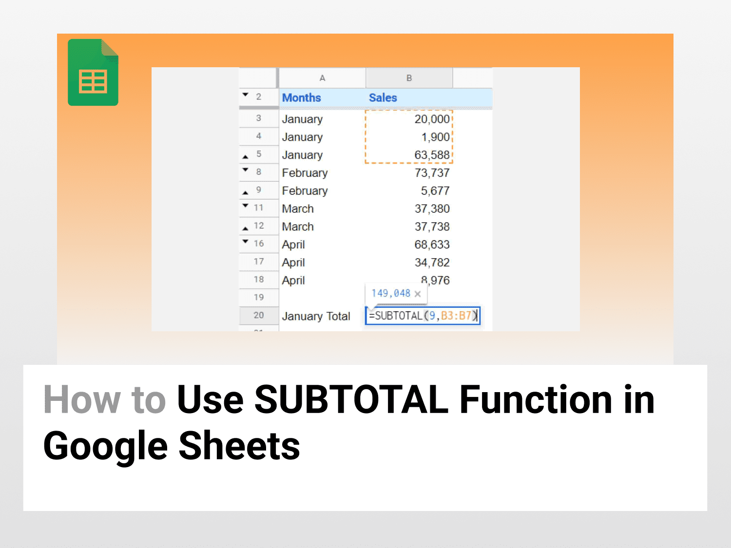
Here is an example of how to use the following syntax:

=SUBTOTAL(9,B3:B7)

Figure 2: Using SUBTOTAL Function in Google Sheets to calculate the Subtotal of January Month Sales

In the above image, function code 9 refers to the summation function for the data range of B3 to B7.

Similarly, the SUBTOTAL Function can be used to calculate the sum of other months as well.

SUBTOTAL Function to exclude Hidden values

Now, this function could have been carried out using the easy-to-use SUM function. But what if there are some hidden rows in the datasheet?

For example, the image given below contains rows that are hidden.

Note: The arrows in the row number panel represent hidden rows.

Figure 3: Using the SUBTOTAL Function to calculate Subtotal of all the rows (including the hidden ones).

By using the SUBTOTAL Function, we can get the total sum of all the rows(including the hidden ones).

We can also exclude the hidden rows using the SUBTOTAL Function by simply prepending the function code with a 10 (in the case of one-digit codes like 6 or 7) and a 1 (in the case of two-digit codes like 10 or 11).

The syntax for summation excluding the hidden ones would be as follows:

=SUBTOTAL(109,B4:B8)

Figure 4: Using SUBTOTAL Function to calculate the Subtotal excluding hidden rows.

Another example of the SUBTOTAL Function has been shown using the following syntax:

=SUBTOTAL(1,B4:B8)

Function code 1 is used for calculating the average of the given range.

Figure 5: Using SUBTOTAL Function to calculate Average for January Sales

The syntax for average operation while excluding hidden rows would now be:

=SUBTOTAL(101,B4:B8)

Figure 6: Using SUBTOTAL Function in Google Sheets to calculate Average excluding the hidden values

Hence, the final value of the filtered data would be distinct from the non-filtered values.

Similarly, just by changing the function codes and range, several functions like calculating the minimum, maximum, product, and so on can be carried out using the SUBTOTAL Function.

SUBTOTAL as a Dynamic Selector

One of the major advantages of the SUBTOTAL function is creating a dynamic selector so that one can choose what function to apply to the dataset.

This can be done by simply following the steps below:

STEP1: Paste the entire codes table on the spreadsheet as given below and select a cell building the dynamic selector. As in our case, the codes are pasted from D21:E31 and the cell for the dynamic selector is A21.

Figure 7: Function Codes to build Dynamic Selector using SUBTOTAL Function

STEP2: Create a drop-down on cell A19 using the Data validation tool.

Data → Data validation

Create the drop-down list using the functions range from the sheet.

Figure 8: Creating a Drop-down in Google Sheets

STEP3: Adding the VLOOKUP syntax with the SUBTOTAL Syntax:

The VLOOKUP formula is used to return the code to the SUBTOTAL function according to the drop-down list item selected.

This is the usual format of the VLOOKUP Syntax:

=VLOOKUP(A19,D19:E29,2,false)

Here, we couple up the VLOOKUP Syntax with the SUBTOTAL Function to achieve the dynamic selector.

Hence, the syntax would be as follows:

=SUBTOTAL(VLOOKUP(A19,D19:E29,2,false),B2:B17)

Figure 9: Using VLOOKUP Syntax with the SUBTOTAL Function in Google Sheets

We can even incorporate another drop-down for a choice to exclude hidden values. This can be achieved using the IF Function:

=IF(A19=”Yes”,0,100)

This basically means that if the value in the cell A19 is “Yes” then 0 is supposed to be used for any further action, else 100 is to be used.

In our case, the total SUBTOTAL Syntax now becomes

=SUBTOTAL(IF(A19=”Yes”,0,100) + VLOOKUP(A20,D19:E29,2,false),B2:B17)

Figure 10: Using IF Syntax to create a drop down for the choice to exclude hidden values

Hence, if “Yes” is selected in the cell A19, 0 would be added to the SUBTOTAL code and this would include the hidden values for the calculations. But if “No” is selected, then 100 would be added to the values, therefore, excluding the hidden values for all the functions.

Hence, this would be the final result.

Figure 11: Building a Dynamic Selector using SUBTOTAL Function in Google Sheets

Conclusion

The SUBTOTAL Function may seem complicated at first, however, once you understand the function codes, you will end up saving a lot of time working on the spreadsheets.

Hopefully, this article helped you understand how to use the SUBTOTAL Function in Google Sheets.

See Also

Want to know more formulas and functions in Google Sheets? Look at our definitive guide on Google Sheets which covers hundreds of such topics here. Enjoy reading!

How to group rows in Google Sheets: Learn how to group rows in Google Sheets. We will also have a look at nested grouping.

Compare Columns in Google Sheets: A 2 minutes easy guide to learn how to compare columns in Google Sheets to look for matching and non-matching values.

Delete Empty rows in Google Sheets: In this article we would see how to delete empty rows in Google Sheets using two different ways.