How to use the QUERY function in Google Sheets

Reading Time: 7 minutes

What it does – Run queries based on an SQL-like Google Visualization API Query Language.

Syntax
=QUERY(data, query, [headers])

data: this is the range of cells to perform queries on.

query: this is the query command to perform. Its value, just like in SQL, must be enclosed in quotation marks or point to a cell containing the appropriate text.

headers: the optional number of header rows at the top of the data.

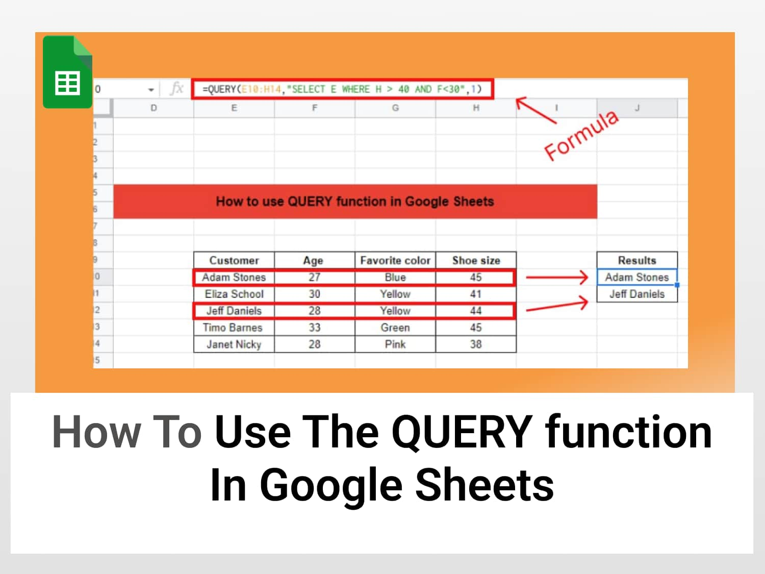
Sample Usage
=QUERY(E10:H14,"SELECT E WHERE H> 40 AND F <30", 1)

//Returns the items from column E whose corresponding value in H is greater than 40 and less than 30 in column F.

=QUERY(E10:H14, "SELECT E,F,G,H ORDER BY F ASC")

//Retrieves the items in columns E, F, G, and H from the range E10:H14 sorted in ascending order according to the values in column F.

Click here to get a copy of the spreadsheet

If you are coming from a programming background or are familiar with databases and SQL, then you know how handy a QUERY command can be. Whether you are one of such experts or are unfamiliar with these concepts, Google sheets QUERY ensures you don’t need to be a guru to do useful work. It lets you perform database manipulations without hassles.

This article will guide you on how to use the QUERY function in Google Sheets to perform “database” operations directly in your worksheets.

• QUERY function
• Syntax
• Parts of the QUERY expression
• QUERY function with SELECT and WHERE
• QUERY function with ORDER BY
• Creating pivot table with QUERY function
• QUERY function with GROUP BY and COUNT
• QUERY function to label a column

What is the QUERY function in Google Sheets?

It is a function that runs a Google Visualization API Query Language across data. It is similar to SQL queries and is a convenient way to sort, retrieve, or manipulate data sets.

Syntax of the QUERY function in Google Sheets

= QUERY(data, query, [headers])

The meaning and significance of each of the arguments of the QUERY function are as follows:

1. Data: this is the range of cells to perform queries on.

• Each data column can contain 5 data types: numeric, boolean, or string values.
• When there are mixed data types in a single column, the majority data type becomes the data type of the column and the minority is seen as null.

2. Query: this is the query command to perform. Its value, just like in SQL, must be enclosed in quotation marks or point to a cell containing the appropriate text.

3. Headers: the optional number of header rows at the top of the data. When it is not provided or set to -1, Google Sheets provides a value based on the content of the data.

Before we go into using the QUERY function it is important to discuss some important components of a typical QUERY expression.

Parts of a QUERY expression:

1. Clause: this is the filter/command that lets you perform certain operations e.g SELECT, WHERE, ORDER BY e.t.c
2. Aggregate functions: these enable us to perform computations or checks on values of interest, which they usually return as single values e.g SUM, COUNT, AVG e.t.c
3. Arithmetic operators: they include operators like +, -, *, and so on. They are used to perform Arithmetic operations.
4. Logical operators: AND and OR can also be used in Google Sheets QUERY to add logical decision-making.

Now that we’ve learned the basics of the QUERY function in Google Sheets, it’s time to head over to where the magic happens – using the QUERY formula in Google Sheets.

How to use the QUERY function in Google Sheets

There are several ways to use the QUERY function and for several purposes. And we will be learning some of its most common usage.s We will be making use of the customer data of a shoe store. Our goal is to retrieve a certain column of the data that match our search criteria. To do this we will use SELECT and WHERE commands.

QUERY function in Google Sheets using SELECT and WHERE

Step 1: set up the data set.

To serve as our database, we are going to fill in the customer information of a shoe store into our Google sheets. Below is the data.

Step 2: Apply the QUERY formula

Go to the formula bar or in any cell of your choice and begin to type in =QUERY Google sheets will suggest a list of formulas, select the QUERY function.

Alternatively, go to Functions ➡ All functions, and scroll down the list to find the QUERY function.

As you can see from the screenshot, Google Sheets is expecting us to provide values for the formula’s parameters.

Now, let us retrieve the names of customers who wear a shoe size greater than 40 and are below 30.

• For the data parameter, we will input A1:A10 as the data range.
• For the query string, enter “SELECT E WHERE H> 40 AND F <30”
• We will use 1 as the header.
• The complete formula is as given below:

=QUERY(E10:H14, "SELECT E WHERE H> 40 AND F <30", 1)

• Press Enter.

The result will be returned according to the parameters we specified in the QUERY formula, as shown below.

The QUERY function returned the names of customers who meet the two criteria we specified — Adam Stones and Jeff Daniels. The SELECT and WHERE commands can be combined in numerous ways depending on what you intend to achieve.

QUERY function in Google Sheets using ORDER BY command

To return a new data set with values arranged in either ascending or descending order, we can use the ORDER BY command. Let us see how.

For instance, using our shoe seller example, let us fetch the names of customers in descending order of age. We want the QUERY function in Google Sheets to look at the age of every customer and organize them from oldest to youngest. We are going to return this data in a new table.

To return the results in descending order, we use the DESC command; to return in ascending order, the ASC command does the job.

The formula for the ascending order is as follows:

=QUERY(E10:H14, "SELECT E,F,G,H ORDER BY F ASC")

Enter the formula and hit Enter.

We have successfully returned customer details in increasing order of their age.

For sorting in descending order, simply replace ASC with DESC.

QUERY function in Google Sheets – Pivot table

Google sheets QUERY function also makes provision for creating a pivot table (average values) from an existing table. We do this using the PIVOT command.

To demonstrate this, we will be adding another column of data to our spreadsheet. This column will denote the gender of the customers. What we are trying to do is, obtain the average age of our customers by sex.

In a new sheet, type in the Google Sheets Query function adding the PIVOT command.

=QUERY(Customers!E19:I23, "SELECT avg(F) PIVOT D)

The results above are the average ages of the customers when considered by their gender.

Query function in Google Sheet using GROUP BY and COUNT

Another interesting way to use the Google Sheets QUERY function is by combining it with the GROUP BY command. With this clause, we can organize data in a preferred way and return them in a different table.

Let us consider another example using our customer data. This time we want to count the number of women we have and return that value in a different table; we will do this for the men, too.

Enter the below formula into a cell of your choice:

=QUERY(Customers!E19:I23,"select I, COUNT (I) GROUP BY I")

Note: The above syntax is for returning the result in a new sheet. If you only want to display the result in the same worksheet, you need only specify the data range without mentioning the name of the spreadsheet.

The result will be returned upon pressing the Enter key, as shown below.

Using QUERY function in Google Sheets and the LABEL clause to title a column.

Sometimes we might want to name/rename a column in our QUERY expression to a title of our choice. We can do this by including a LABEL clause directly in the formula. When the data is retrieved it will appear under a column with our preferred title.

The LABEL clause has a simple syntax – LABEL X ‘preferred name’

Where X is the range of data to be returned in a table.

Let us title the column which holds our customer’s sex. We will set the preferred name to SEX.

Conclusion

There are several Query commands and nearly limitless ways to utilize the QUERY function in Google Sheets in performing operations on data sets.

For a more comprehensive tutorial on the QUERY function in Google Sheets, check out this article.

See also

There are plenty of other useful tutorials with tips and tricks on Google Sheets. You can find them all here.

Here are some similar articles you may find interesting:

https://blog.tryamigo.com/sort-query-using-order-by-in-google-sheets/

https://blog.tryamigo.com/google-sheets-pivot-query-in-google-sheets/

https://blog.tryamigo.com/how-to-eliminate-duplicates-in-google-sheets/