What it does – It lists all the Sundays between any two dates in Google Sheets
Syntax:=query(ArrayFormula(TO_DATE(row(indirect("E"&Start_Date):
indirect("E"&End_Date)))), "Select Col1 where
dayOfWeek(Col1)=1")
We can pass by value as shown:=query(ArrayFormula(TO_DATE(row(indirect("E"&"01/01/2022"):
indirect("E"&"03/04/2022")))), "Select Col1 where
dayOfWeek(Col1)=1")
//This returns the list of Sundays falling between 01/01/2022 and 03/04/2022
We can also pass by reference as shown:=query(ArrayFormula(TO_DATE(row(indirect("E"&A4):
indirect("E"&B4)))), "Select Col1 where
dayOfWeek(Col1)=1")
// This returns the list of Sundays falling between the value stored in A4 and the value stored in B4
Sample Google Sheets template with formula here.
Google Sheets offer a variety of tools that you can use to your advantage. Do you know how to list all Sundays between two dates in Google Sheets? It might seem to be tricky but the procedure is quite simple and easy to implement.
An organization is operating on all the days except Sundays and it wishes to list all the non-operational days. In that scenario, we will have to list all Sundays between two dates. To be able to perform a task like this, we will learn how to list all Sundays between two dates in Google Sheets.
Prerequisite functions
Before beginning the tutorial, we need to learn about a few functions that will be used in our formula. Understanding these functions will give you a better grasp of the tutorial. Then you will be able to learn about how to list all Sundays between two dates in Google Sheets.
Query function in Google Sheets
The QUERY function in Google Sheets empowers you to execute queries written in an SQL-like language. These queries allow you to perform database-type searching in Google Sheets, so you can find, filter, and format data with maximum versatility. The syntax of the Query function is as follows:
=QUERY(data, query, [headers])A brief description of the syntax is as follows:
- Data: The range of cells/data to perform operations on
- Query: The query to perform i.e. a conditional statement to fine, filter, or format data
- Headers: The number of header rows at the top of the range. It’s optional as in most cases the Query function in Google Sheets can automatically detect it.
Array Formula function in Google Sheets
An array formula is a formula that can perform multiple calculations on one or more items in an array. Array formulas can return either multiple results or a single result. The syntax of the Array formula is as follows:
=ARRAYFORMULA(array_formula)Array_formula: This parameter can either be:
- a range
- a mathematical expression using one cell range or multiple ranges of the same size
- a function that returns a result greater than one cell
To_Date function in Google Sheets
The To_date function in Google Sheets converts a numerical value to a date interpreting the value as the number of days since 30-Dec-1899. A positive parameter stands for the date beyond 30-Dec-1899 and a negative parameter stands for the date before the same. The syntax of the To_Date function is as follows:
=To_Date(x)A brief description of the syntax is as follows:
- X stands for a numerical value, it can also be a fraction
- That means =to_date(0) returns the above date and =to_date(1) returns 31-Dec-1899
- Negative values like =to_date(-1) are interpreted as days before this date.
- Fractional values like =to_date(2.5) are interpreted as 01/01/1900 12:00:00 pm
Row function in Google Sheets
The ROW function in Google Sheets returns the row number of a given cell. For example, if you want to know what row number cell A1 is in, you would use the function. This function is especially useful when you’re working with formulas and need to refer to specific rows or columns. The syntax of the Row function is as follows:
=ROW(x)X: The value of cell reference whose row number will be returned
Indirect function in Google Sheets
The indirect function in Google Sheets returns the cell reference specified by a string. It is used when you want to change the reference to a cell within a formula without changing the formula itself. The syntax of the Indirect function is as follows:
=INDIRECT(Cell_reference_as_a_string)Here the “cell_reference_as_string” means a cell reference written as a string. For example, A1 is a cell reference. If you enter this cell reference as “A1”, it’s called cell reference A1 ‘written as a string’. You can replace the formula or say cell reference A1 with =INDIRECT(“A1”). Both of them are the same.
We will not start learning about how to list all Sundays between two dates in Google Sheets.
List all Sundays between two dates in Google Sheets
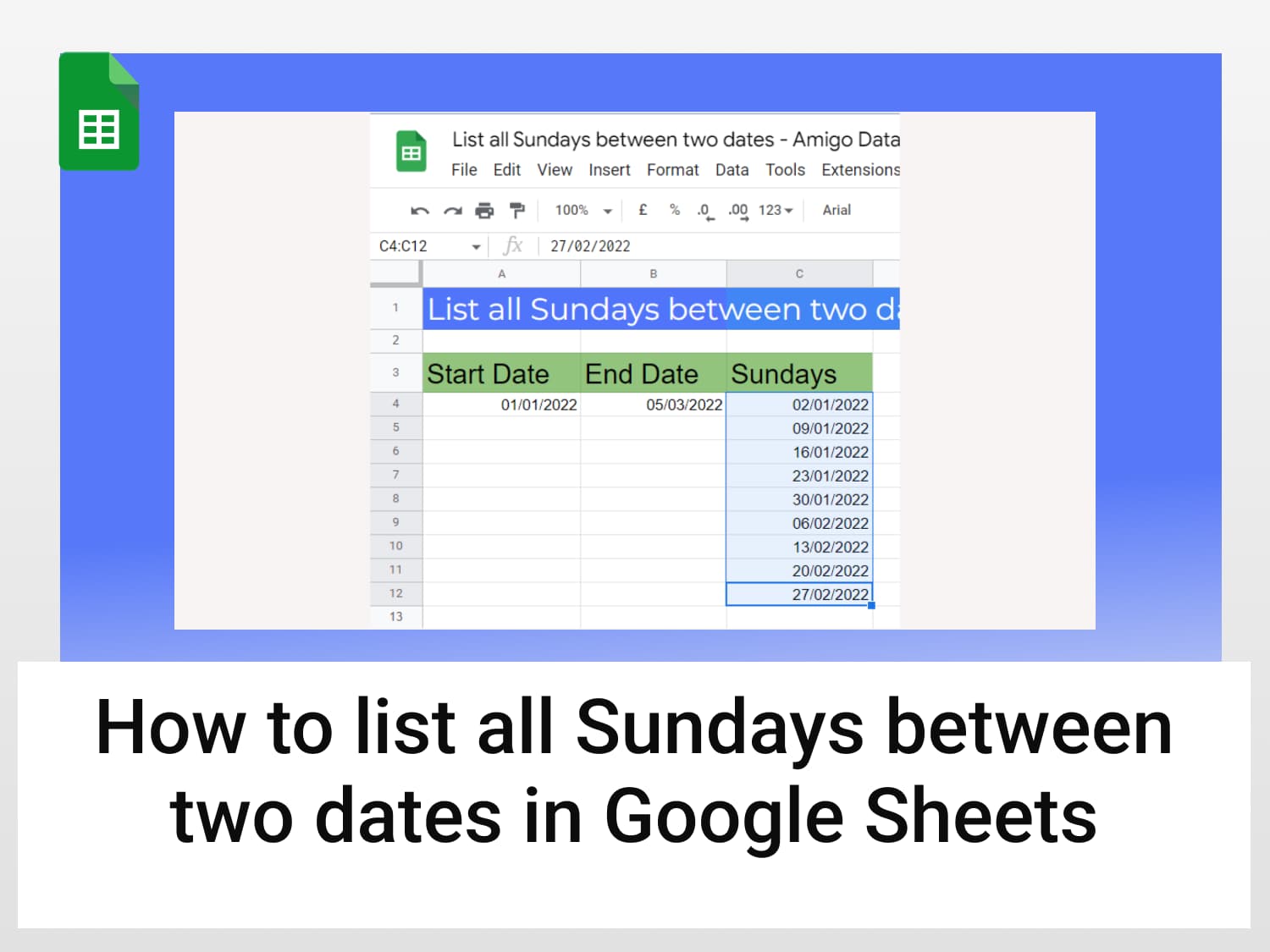
We are now equipped with the knowledge of various functions which we will use. In the following example, there is a start date and an end date. Our objective is to list all Sundays between two dates in Google Sheets.

In this tutorial, we will list all the Sundays between two dates in Google Sheets. The steps are as follows:
- Select the empty cell under the Sunday header
- We will use ArrayFormula to populate all the dates between the start and end date. We will then use the query function to sort all the dates that belong to Sunday. Type in the following formula:
=query(ArrayFormula(TO_DATE(row(indirect("E"&A4):indirect("E"&B4)))),"Select Col1 where dayOfWeek(Col1)=1")
- Hit Enter and you will see the list of Sundays between two dates in Google Sheets

- The list of dates is in DateValue form. We need to change it to the date form. Select the entire column

- Click on the Format menu and select the Number option. Then further select the Date option

- You will now see the DateValues in the date form

We have successfully learned how to list all Sundays between two dates in Google Sheets. The formula used here is quite simple and generalized. It can be used as it is, just make sure to enter the correct cell addresses of the start and end dates.
Conclusion
We have successfully learned how to list all Sundays between two dates in Google Sheets. We have gone through a step-by-step process along with a detailed explanation of the functions involved in the complete process. You can now easily list all Sundays between two dates in Google Sheets.
See Also
You have successfully learned how to list all Sundays between two dates in Google Sheets. Are you interested in learning more about how much you can succeed with Google Sheets? With so many powerful features of Google Sheets, you save time and effort.
We have several tutorials that cover tricks and tips in Google Sheets. You can discover them here.
Here are some articles you might be interested in:
https://blog.tryamigo.com/how-to-create-a-countdown-timer-in-google-sheets/
https://blog.tryamigo.com/sort-query-using-order-by-in-google-sheets/
https://blog.tryamigo.com/introduction-to-date-function-in-google-sheets/