What it does: returns the largest numeric value that meets one or more criteria in a range of values
Syntax
=MAXIFS(range, criteria_range1, criterion1, [criteria_range2, criterion2, …])
range is the range of cells from which the maximum value is to be found.
criteria_range1 is the range of cells over which to evaluate criterion1.
criterion1 is the condition to apply to criteria_range1.
[criteria_range2, criterion2, …] are optional additional ranges and their associated criteria.
Sample Usage
=MAXIFS(B2:E20,A2:A20,”man”)
./retrieves the highest number in range E4:E20 while matching the entry F8 in range C4:C20.
Sample Google Sheets template with formula here.
The MAXIFS function is a combination of two functions: the MAX function and the IF function. The MAXIFS function can be used with criteria based on dates, numbers, text, and other conditions.
The MAXIFS function can be used in various scenarios such as finding the highest marks scored by a student in a specific subject, the highest recorded temperature of a particular city or country, identifying the country with the maximum sales of a product or a service, and so on.
Formula for the MAXIFS function in Google Sheets
=MAXIFS(range, criteria_range1, criterion1, [criteria_range2, criterion2, …])Where the argument:
- range is the range of cells from which the maximum value is to be found.
- criteria_range1 is the range of cells over which to evaluate criterion1.
- criterion1 is the condition to apply to criteria_range1.
- [criteria_range2, criterion2, …] are optional additional ranges and their associated criteria.
Things to note:
MAXIFS will return 0 if none of the criteria is satisfied.
Range and all of the criterion ranges must be the same size, otherwise the MAXIFS will return a #VALUE error.
How to use the MAXIFS function in Google Sheets
To use the MAXIFS function in Google Sheets, follow these steps:
- Type =MAXIFS into the cell of your choice
- Select the range to draw the maximum number from
- Enter the criteria range
- Specify the criteria, enclose the formula and press Enter
In order to better understand how to use the MAXIFS function, let’s consider a few examples.
Let us take the weightlifting record of the last Summer Olympics for both men and women together in an unorganised manner, as shown below.

You make a copy of the Google Sheets template for hands-on practice.
In order to find the highest weight lifted by a man using the MAXIFS function, we use the following formula:
=MAXIFS(E4:D20,C4:C20,"Man")This will return the maximum weight lifted by the men, which is 488 in this case.

To make the formula more versatile, we can specify a cell as the criterion in the formula. We can then enter the search parameter into the cell and the answer will be shown in the formula cell.
In the above example, we can replace “Man” in the formula with C22. Entering “Man” in cell C22 will give the result of the highest record for men and entering “Woman” will return the maximum record for women.

MAXIFS function in Google Sheets with multiple criteria
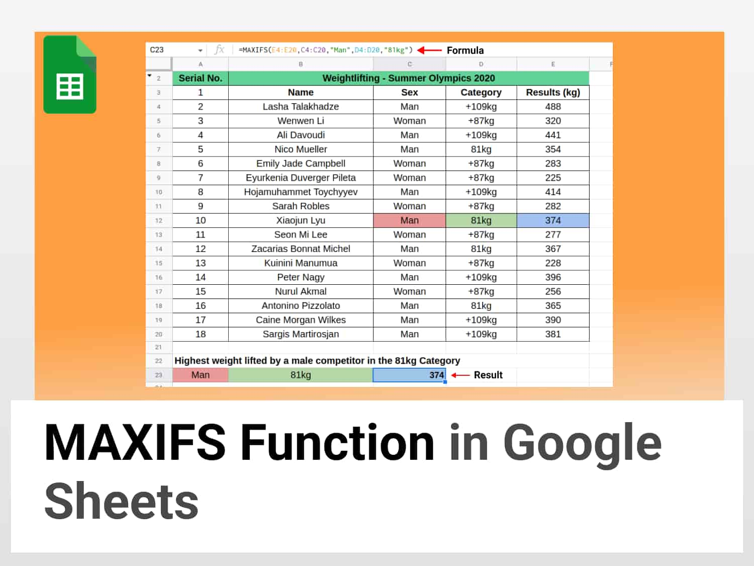
The MAXIFS function can be used with multiple conditions. In our weightlifting data, suppose that we want to find the highest weight lifted in the Men’s 81kg Category, we use the following formula:
=MAXIFS(E4:E20,C4:C20,"Man",D4:D20,"81kg")This will return 374 as the result, the highest value in the Men’s 81kg Category, as per our data.

Like in the case with the first example, we can specify blank cells in the formula instead of the range criteria (“man” and “81kg”) which will point to the cell with the search value according to our input.
MAXIFS function in Google Sheets with operators as criteria
Tip: The MAXIFS function supports logical operators (>,<,<>,=).
We can be more specific with our search by specifying the criterion with an operator. Suppose that we want to find the highest weight lifted after 488, by either men or women. We can accomplish this by using either the “Not equal to” operator (“<>”) or the “Less than” operator (“<”).
Logical operators in Google Sheets:
- Equal to (=)
- Not equal to (<>)
- Less than (<)
- Greater than (>)
- Less than or equal to (<=)
- Greater than or equal to (>=)
Let us do it with the “Less than” operator.
We need to specify the range from which the result is to be returned, and specify also the range from which we want to exclude the value from and add the operator.
The formula is:
=MAXIFS(E4:E20,E4:E20,"<488")This will return the highest value less 488, which is 441 in our example.

We can also separately find out the second highest record for both men and women by filtering the highest records for men as well as women by using the “Not equal to” or the “Less than” operator. Let us consider with an example, this time using the “<>” operator.
The formula is as given below:
=MAXIFS(E4:E20,C4:C20,C22,E4:E20,"<>488",E4:E20,"<>320")Here, C22 is the cell in which to enter the search key, ie, “Man” or “Woman”, E4:E20,”<>488” indicates that we want the formula to ignore 488 for men from the range, and E4:E20,”<>320” likewise for women.
On entering “Man” in cell C22, we get 441 as the answer, which is the largest number excluding 488.

Entering “Woman” returns 283 as the result, the highest number after 320.

Conclusion
The MAXIFS function in Google Sheets is a very useful tool to quickly find out the highest value from a given range of cells specified by a given set of criteria or conditions. Multiple criteria can be assigned to the MAXIFS function to find more specific values.
See also
Use AVERAGEIF Function in Google Sheets | Latest Guide
How to Use the WEEKDAY Function in Google Sheets – Easy Guide
How to Use the CHOOSE Function in Google Sheets – Easy Guide