What it does – Calculate the sum of the product of two corresponding data ranges that are of equal size.
Syntax=SUMPRODUCT (array1, [array 2,...])array1: The primary array whose entries the function will multiply by corresponding entries in another array.array2: [Optional] The secondary array that the function will multiply by array1.
Sample Usages=SUMPRODUCT(A2:A8, B2:B8)//Calculates the sum of the ranges A2:A8 and B2:B8 and returns their product.=SUMPRODUCT(A2:A8 > 4, B2:B8)//Calculates the sum of all data in the range A2:A8 with values greater than 4, then multiplies the corresponding values in the range B2:B8.
Get the spreadsheet template with the formulas here.
Some formulas provide us with an excellent and convenient way to perform interesting operations. The SUMPRODUCT function in Google Sheets is one such functions.
This tutorial is intended as an easy guide for using the SUMPRODUCT formula in Google Sheets for basic to more complex operations.
- SUMPRODUCT function
- Using the SUMPRODUCT function
- SUMPRODUCT with condition
- SUMPRODUCT with multiple conditions
What is the SUMPRODUCT function in Google Sheets?
The SUMPRODUCT formula calculates the sum of the product of two corresponding data ranges that are equal in size. It considers multiple data entries in a given array/range and sums the product of corresponding entries. It can handle datasets of up to 255 arrays.
It is useful in cases where we want to first perform multiplication and then return the sum of the resultant data.
Note: Arrays must be of equal size. The Sumproduct function can only operate on data ranges that are equal in length. It will return an error if the arrays are of unequal sizes.

Consider the table above, a coffee shop recently purchased different types of mugs, all of the different prices and in different quantities.
To calculate the total amount spent on the entire set of mugs, one would ordinarily get the sum of all values of the first column and multiply it with the second.

And then manually add the results of the multiplication.

The SUMPRODUCT function in Google Sheets eliminates this laborious approach and provides an elegant way to do similar operations and more.
You can use the SUMPRODUCT function to perform simple SUM operations if only one array is supplied.
How to use the SUMPRODUCT function in Google Sheets
The SUMPRODUCT function in Google Sheets is a simple function needing just a few parameters, though it can be applied to much more complex scenarios. This example shows a basic application.
SUMPRODUCT function in Google Sheets basic example
Step 1: Setup the data
To use the SUMPRODUCT function in Google Sheets let us consider the following dataset of the coffee shop mentioned earlier.

We are going to perform the same operations as before, only much more elegantly this time around.
Step 2: Apply the SUMPRODUCT formula
In the cell below the total price, begin to type the formula, then select it when Google Sheets brings up suggestions.
=SUMPRODUCT (array 1, [array 2,...])Alternatively, you can select the formula from the function menu. Go to functions→ all functions→scroll down to find SUMPRODUCT.
For array 1, we will use A6:A11 as the data range.
For array 2, we use B6:B11 as the range.

Hit Enter.

The function automatically calculates and returns the same value we got in our manual technique, but this is a much faster and neater way to do this.
The SUMPRODUCT function in Google Sheets is not just limited to simple addition and multiplication. We are going to look at more technical applications in the course of this guide.
Tips:
↠ SUMPRODUCT adjusts its values with the addition of new records. Hence, no need to manually compute values like in the old method. All we need to do is adjust the parameters to include the new range.
↠ You can also add numerous arrays to the sheet and the SUMPRODUCT function will compute the values of the new data set.
SUMPRODUCT IF
SUMPRODUCT function in Google Sheets supports the use of conditional statements. That is, we can provide rules, so to speak, which the formula has to observe. And based on these rules, the formula can return the data that matches our condition.
When combined with conditional statements the SUMPRODUCT function in Google Sheets can become a very powerful formula. We can filter through large data sets and only compute values for fields we are interested in.
So how do you use the SUMPRODUCT function in Google Sheets with conditions?
How to Use the SUMPRODUCT function in Google Sheets with conditions
Let us once again go back to our coffee shop. Let’s say our coffee shop owner wants to only see values for mugs that they purchased in quantities greater than 4 so that she can decide if buying in large numbers saves money. We are going to use a logical statement to do this.
A simple conditional flow goes — return coffee mug cost if its quantity > 4.
Apply this conditional flow to the SUMPRODUCT FORMULA:
=SUMPRODUCT (A6:A12 > 4, B6:B12)
The function computed values for only coffee mugs that met the criteria skipping cells A8, A9, and A11 which do not.
We can use this to sort through huge sets of data in much more complex setups with ease.
How to use the SUMPRODUCT function with multiple conditions example
We can also apply conditionals to multiple arrays at once, e.g return coffee mug if quantity is > 4 AND colour = brown. We will add an extra column to our table for the colour of the mugs purchased and we will return values for only brown ones.
To add a new column simply right-click on the selected column (column C)
Select insert 1 column to the right.

We will name this column Colour. Fill the column with the data below.

Then enter the formula below.
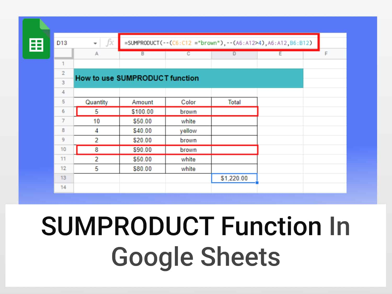
=SUMPRODUCT(--(C6:C12 ="brown"),--(A6:A12>4),A6:A12,B6:B12)To perform logical loops we will use the double minus “–” operator and specify the conditions in brackets. As can be seen from the above, we have two major conditions :
- Check to see if the colour of the mug is brown
- The second bracket checks to see if the quantity is greater than 4.
Hit enter.

The SUMPRODUCT function successfully calculates the values for mugs that are brown and were purchased in more than 4 units i.e (5×100) + (8×90) = 1220.
Conclusion
The SUMPRODUCT function greatly simplifies certain operations that would otherwise be tedious to perform manually. Once you understand how to use conditional statements properly—which I hope you do now— you can leverage the formula in unique ways to solve complex problems.
See also
Check out some of our articles on other interesting topics about Google Sheets.
https://blog.tryamigo.com/sumifs-function-in-google-sheets-quick-guide/
https://blog.tryamigo.com/how-to-use-subtotal-function-in-google-sheets/
https://blog.tryamigo.com/calculate-weighted-average-in-google-sheets/