How to Use SWITCH Function in Google Sheets for 2022 | Expert Guide 💻

Reading Time: 4 minutes

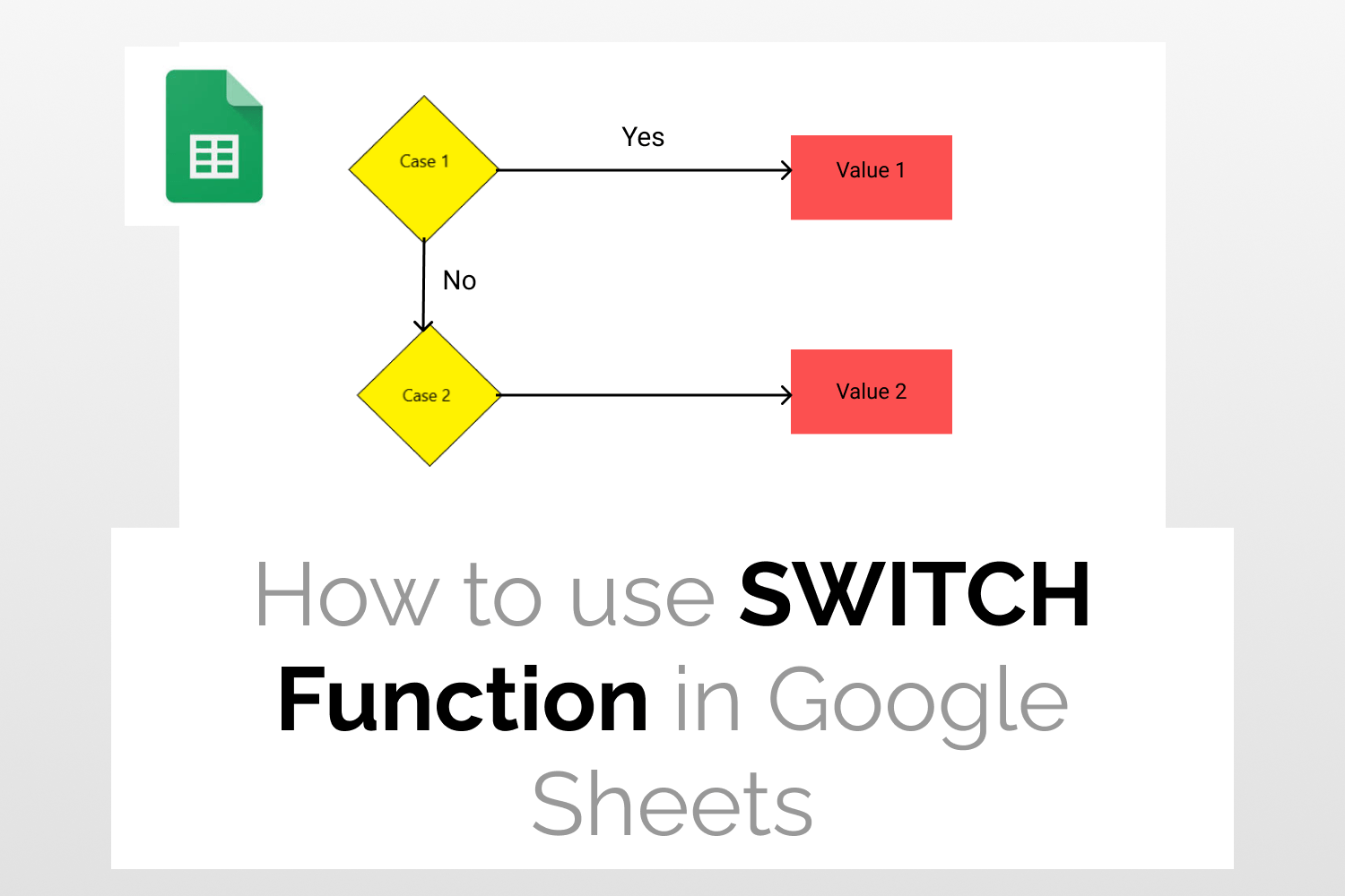
What it does – It compares a specified expression with a list of conditions and returns a value corresponding to the first match found. In case no match is found, the function returns an optional default value.

Syntax
SWITCH(expression, case1, value1, [case2, value2, ...], [default])

expression – This can be a value, expression or reference to a cell or range of cells containing a value or expression.

case1, case2…. – These are the cases against which the value of the expression will be checked. 

value1, value2…. – These are the values to be returned if the corresponding case finds a match. 

default – This is an optional value to be returned if none of the cases match the expression.

Sample Usage
=SWITCH(A2, "A", "Excellent", "B", "Satisfactory", "C", "Average", "D", "Needs Improvement", "E", "Fail")

//This returns “Excellent” as the answer if the value in A2 is “A”, “Satisfactory” if “B”, and so on.

Objective

Learn how to use the SWITCH function in Google Sheets.

Introduction

The SWITCH Function in Google Sheets compares a specified expression with a list of conditions and returns a value corresponding to the first match found. In case no match is found, the function returns an optional default value. The SWITCH Function in Google Sheets is a good option to use when you have to check multiple criteria against a given value. 

The SWITCH function is a bit similar to the nested IF function but easier to read!

Syntax

=SWITCH(expression, case1, value1, [case2, value2, ...], [default])

• expression- This can be a value, expression or reference to a cell or range of cells containing a value or expression. 
• case1, case2….- These are the cases against which the value of the expression will be checked. 
• value1, value2….- These are the values to be returned if the corresponding case finds a match. 
• default– This is an optional value to be returned if none of the cases match the expression.

Using the SWITCH Function 

Example 1

Step 1: Enter the data 

The spreadsheet below lists the grades scored by students in an examination. Based on the grades we need to fill the remarks column using the following categorization- 

A-> Excellent

B-> Satisfactory

C-> Average

D-> Needs Improvement 

E-> Fail 

Let’s have a look at how to do this 

Step 2: Use the SWITCH Function formula 

To fill in the remarks column, I first select a cell and type in the following formula

=SWITCH(A2, "A", "Excellent", "B", "Satisfactory", "C", "Average", "D", "Needs Improvement", "E", "Fail")

As you can see, the respective remarks get inserted in the chosen cell. 

Similarly, we can fill the remaining cells by applying the SWITCH Function formula. 

Example 2 

Step 1: Enter the data 

I have added another list to the previous example spreadsheet for this example. This list specifies the grade awarded to each student. Now we need to assign a remark to each student’s performance based on the grading scheme.

Let’s see how to do this in the next step. 

Step 2: 

I first select a cell to fill in the remarks. Next type in the following formula 

=SWITCH(B2,E2,F2,E3,F3,E4,F4,E5,F5,E6,F6,"Invalid Grade")

In the formula above I have also added a default value of “Invalid Grade”. If any grade other than A, B, C, D or E is assigned to a student then the grade is invalid and the value “Invalid Grade” is displayed in the remarks column. 

The corresponding remark is displayed in the selected cell. 

In a similar manner, we can add the remarks for the remaining students as well. 

Why am I getting #NA error?

The #NA error is displayed when the SWITCH Function doesn’t find a case to match with the expression. To avoid getting this error, you should define the default value argument of the SWITCH Function. 

Conclusion

Hopefully, you were able to learn how to use the Switch function in Google Sheets to change the value in one cell based on another. One limitation is that you cannot use greater than or less than operators because the Switch function in Google Sheets can only work with exact matches.

If you enjoyed reading this article, you might like our Definitive Guide on Google Sheets which has been created by experts to solve hundreds of doubts related to using Google Sheets.