What it does – It computes the linear trend (slope and y-intercept) using the least-squares method
Syntax:=LINEST(known_data_y, [known_data_x], [calculate_b], [verbose])known_data_y – It refers to the array or range containing dependent values already known.known_data_x – It refers to the values of independent variables that correspond with known_data_y.calculate_b – It is an optional argument that calculates the y-intercept (b). If FALSE, the function forces b to be 0, which forces the line to pass through the origin.verbose – It is an optional argument that specifies whether to return more regression properties. By default, it is set to FALSE. If the verbose argument is TRUE, the LINEST function also returns a standard error, coefficient of determination, f-statistic, degrees of freedom, regression sum of squares, and residual sum of squares.
Sample usage:=LINEST(A4:A17, B4:B17, FALSE, FALSE)
//This calculates slope and y-intercept of the regression line passing through the origin
Sample Google Sheets template with formula here.
Google Sheets offer us a wide range of tools to analyze the given data. One of the best ways to analyze data is by using linear regression which helps us to establish a trend and make predictions. In such scenarios, the LINEST function in Google Sheets can come in handy.
Let’s learn how to use the LINEST function in Google Sheets. The article comprises of the following sections
What is the LINEST function in Google Sheets?
The LINEST function in Google Sheets is used to perform the linear regression analysis on a given dataset. Linear regression allows us to fit a straight line through the given data points in such a way that mean squared error is minimized.

The linear regression equation is in the form ‘y= bx + c’. The variable ‘x’ refers to the independent variable, and ‘y’ is the dependent variable. The letter ‘b’ is the slope of the line, and c indicates the y-intercept.
Let’s say there is a scenario where we have been given a dataset full of ‘x’ and ‘y’ values and we have to predict the value of ‘y’ for a given value of ‘x’. In such scenarios, it becomes important to use linear regression analysis to predict the value of the unknown variable. That’s why it’s important to learn how to use the LINEST function in Google Sheets.
The LINEST function in Google Sheets
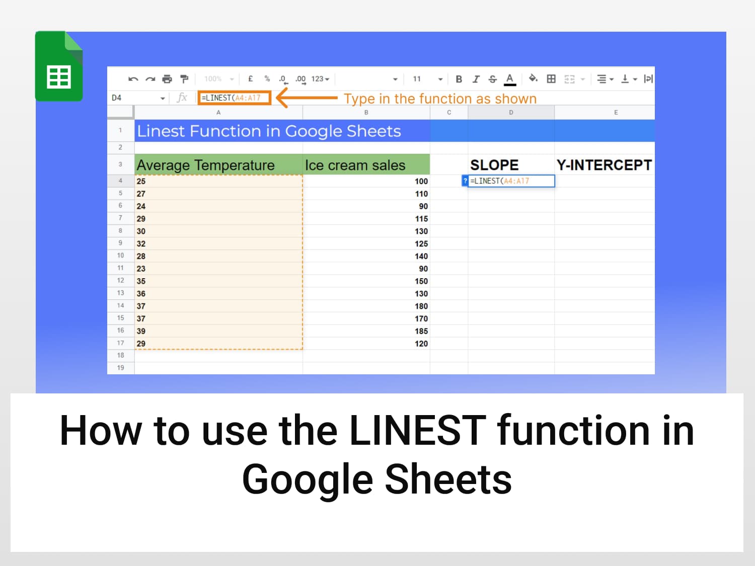
In the following example, we are going to learn how to perform linear regression analysis on a given dataset using the LINEST function in Google Sheets. We have a dataset having x and y values where x stands for average temperature throughout the day and y stands for daily ice cream sales.

Our objective is to find out the relationship between ice cream sales and average temperature throughout the day. We can do this by simply applying the regression analysis using the LINEST function in Google Sheets. The step-by-step process is as follows:
- Select the empty cell under the SLOPE header as shown.

- Begin your function with the ‘=’ sign. Type in the ‘LINEST’. The Google Sheets will prompt this function, press the Tab/Enter key to autocomplete. The tooltip guide will appear along with the details.

- Enter the first parameter that is the dataset under the Average Temperature header

- Enter the second parameter that is the dataset under the Ice cream sales header

- The next parameter will have a TRUE value as we don’t want to force the regression line to pass through the origin

The next parameter will have a FALSE value as we don’t require additional data as of now. The final formula should look like this:
=LINEST(A4:A17, B4:B17, TRUE, TRUE)
- Press the Enter key and the values of the slope and y-intercept will be displayed in the respective cells. Using the slope and y-intercept we can easily construct a regression line or predict the value of an unknown variable.

- The value of the slope and y-intercept of the regression line gets displayed under their respective headings.
We can now simply calculate the ice cream sales if we have the value of average temperature and vice versa. For example, if we wish to calculate the ice cream sales for a day with average temperature of 20 degrees Celsius. In that case, we can simply calculate the value using the following formula:
Average temperature = slope * ice cream sales + y-intercept
20 = 0.15 * ice cream sales + 10.35
Ice cream sales = 9.65/0.15 = 64
- If we had entered the value of the 4th parameter as TRUE then the LINEST function would have returned additional values as follows:

- The slope (gradient) of the line is 0.1555682958
- The y-intercept which is the value of y when x=0 is 10.395
- The standard error value for the slope value is 0.01983706856
- The standard error value for the y-intercept is 2.667
- The coefficient of determination is 0.836738495
- The standard error for the y estimate is 2.214
- The F statistic is 61.50171126
- The number of degrees of freedom is 12.000
- The regression sum of squares is 301.5246934
- The residual sum of squares is 58.832
Conclusion
We have successfully implemented the LINEST function in Google Sheets and have learned how to successfully perform linear regression analysis on a given dataset. We have also understood that we can gather additional statistical information by simply checking the verbose option as TRUE. You are now all set to use this tool to your advantage.
Commonly asked questions
How do you force a trendline through Origin in Google Sheets?
One can force the trendline through the origin by entering the value of the 3rd parameter (calculate_b) as FALSE
Can Google Sheets do a line of best fit?
You can do this in Sheets through an option in the chart editor. After making a scatter plot, you can add a line of best fit by opening the chart editor by clicking the three dots in the top right corner. Once the chart editor is open, make sure customize is selected.
Can you add a trendline in Google Sheets?
You can add a trendline to each series of data by going to the Chart Editor, Customize, then Series. On the drop-down menu, make sure the series you want to add a trendline to is selected. To add a trendline, check the box next to the trendline type you want to use.
See Also
We have learned how to use the LINEST function in Google Sheets. Are you interested in learning more about how much you can succeed with Google Sheets? With so many powerful features of Google Sheets, you save time and effort.
We have several tutorials that cover tricks and tips in Google Sheets. You can discover them here.
Here are some articles you might be interested in:
https://blog.tryamigo.com/find-the-line-of-best-fit-in-google-sheets/
https://blog.tryamigo.com/how-to-perform-linear-regression-using-google-sheets/
https://blog.tryamigo.com/introduction-to-date-function-in-google-sheets/