What it does – To perform a vertical lookup on the set of data filtered using the IF function
Syntax:
=VLOOKUP(search_key, IF(logical_expression, value_if_true, value_if_false), index, [is_sorted])
search_key - It refers to the value the function searches for. It can be a number, text, or a reference

range - It refers to the dataset, this is the table in sheets we want to look through. Its first column is where the search key parameter is usually taken from. This can be a range of cells or a function that returns a range.

index - It refers to the column index of the value to be returned by the vlookup function

is_sorted - It determines whether to look up the exact or approximate value. FALSE returns the exact match; TRUE the approximate match.

Sample usage:
=VLOOKUP(J7, IF(J6=“Royal Place”, B5:C12, E5:F12), 2, 0)
//What this formula does is look up for "Royal Place" and then returns the corresponding value from the range B5:C12 if yes; otherwise it returns the value from the second range, E5:F12.
Sample Google Sheets template with formula here.
When it comes to searching through rows and columns of data for an entry, especially in a large data set, the VLOOKUP formula in Google Sheets is one useful tool that enables us to do otherwise difficult tasks.
VLOOKUP means vertical lookup. It provides a convenient method for retrieval of data by looking up keys in the column of interest, this key is usually an entry in the first column of the table and it helps us find specific data in the corresponding row.
However, the VLOOKUP function has limitations when it comes to how it can retrieve data.
This guide aims to demonstrate how to use VLOOKUP with IF function in Google Sheets to perform operations beyond what the VLOOKUP formula is normally used for.
Note that the VLOOKUP function doesn’t support search keys based on regular expressions. This is a major limitation in Google Sheets. There is no room for making conditional statements by default, hence we need to combine it with another Google Sheets function — the IF function.
Why combine the VLOOKUP with IF function in Google Sheets
The VLOOKUP function is used to lookup for values in a table and the IF function to obtain the ability to return values based on criteria we specify. Combining the two improves the VLOOKUP formula and enables us to do more with it.
Consider the table below that represents different prices for the same foods in two different restaurants.

Retrieving the price of a specific food in one table using VLOOKUP would be very straightforward as all we need to do is provide the parameters – Food name, Data range e.t.c
But what if we instead wanted a way to quickly switch between both restaurants to check the price of pizza in them? Or if we wanted to check if food is ready based on the time an order was placed? These are things we, unfortunately, cannot easily do with the VLOOKUP formula, recall that it doesn’t support regular expressions by default.
In the following example, we will use the VLOOKUP formula differently by combining it with the IF function in Google Sheets. This will enable us to retrieve foods and their prices based on the conditions we will specify.
How to use VLOOKUP with IF function in Google Sheets
There are a couple of ways to use both Google Sheets functions together. First, let us take a look at the IF function in Google Sheets.
Syntax of the IF function
=IF(logical_expression, value_if_true, value_if_false)- logical_expression is an expression or reference to a cell containing an expression that evaluates to TRUE or FALSE.
- value_if_true is the value the IF function returns if logical_expression is TRUE.
- value_if_false is an optional value to return if logical_expression is FALSE. This is blank by default.
Example 1: Use VLOOKUP with IF function in Google Sheets to perform a lookup in 2 tables
Back to our restaurant, to use VLOOKUP and the IF function in Google Sheets to check both tables for the price of a pizza, and return the prize for the particular restaurant we want, we will use the formula below:
=VLOOKUP(J7, IF(J6 = "Royal Place",B5:C12,E5:F12), 2, 0)The formula and how to implement is explained in steps hereunder:
- Provide the required parameters of the VLOOKUP function in Google Sheets.
- Supply the IF function as the second parameter of the VLOOKUP function (the range) and specify the conditions you want to be met.
- Since the prices are listed in the second column, we enter the index as 2.
- The sort value is 0, meaning that we want the exact value to look up for.
The conditions here are simple: If “Royal Place” is the specified restaurant, return its data, else return the data for the second restaurant.
Note: the IF function returns a range of cells. Recall that the range parameter of the VLOOKUP in Google Sheets can be direct values or references to other cells.

Example 2: Use VLOOKUP and IF function with comparison operators
Comparison operators such as the greater than > and less than < let us compare different expressions or values and return TRUE or FALSE. They are very useful in conditional statements.
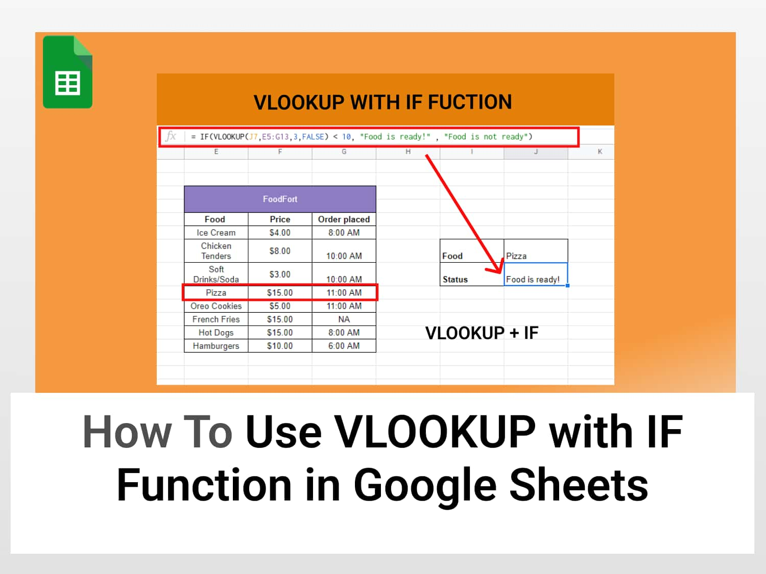
Now, let us determine when a particular food would be ready. To do this we have slightly modified our table by adding a third column. This column represents the specific time a customer placed an order.

Assuming every order placed before a given time is ready for pickup but those placed after that time isn’t. We can easily model this condition as follows :
= IF(VLOOKUP(J7,E5:G13,3,FALSE) < 10, "Food is ready!" , "Food is not ready")- We evaluate the return value of the VLOOKUP formula by checking if the time is lower than 10 am.
- If it evaluates to TRUE, the function returns “food is ready” If FALSE, “food is not ready”.

The image above shows that the pizza is ready for pickup.
Example 3: Use VLOOKUP and the IF function to modify error messages
When we try to retrieve invalid data e.g a particular food that is not in the table, we are met with the #N/A (not available) error message.

We can modify this to return a custom message instead of the #N/A error, to do this, we will use the ISNA function in combination with VLOOKUP and IF functions
Enter the formula below into a cell
=IF(ISNA(VLOOKUP(I8,E7:F14,2,0))=TRUE,"Will be available by 12pm today",VLOOKUP(I8,E7:F14,2,0))
Instead of returning an NA error, we have set the VLOOKUP to return a different message when it cannot find a particular food.
Conclusion
Combining VLOOKUP with IF function in Google Sheets ensures we get to perform more sophisticated lookup tasks in our spreadsheet as we have seen in this tutorial.
Frequently Asked Questions
Can you do VLOOKUP in Google Sheets?
Yes. Google Sheets has the VLOOKUP formula similar to that in excel. You can perform all kinds of vertical lookup operations using the VLOOKUP in Google Sheets. To further extend its use you can combine it with the IF function as we demonstrated in this tutorial.
Can you VLOOKUP from another sheet in Google Sheets?
Yes, it is very easy to retrieve data from a table in another sheet. All you need to do is change the range parameter to reference the table in the other sheet you want to lookup
For instance, from Sheet2 you can retrieve data from Sheet1 using the formula:
=VLOOKUP (A1, Sheet1!A3:D9, 2, 0)
See also
We have other interesting articles on using the VLOOKUP formula in Google Sheets, check them out
VLOOKUP from another sheet in Google Sheets