What it does – Calculates the internal rate of return of an investment based on a specified series of potentially irregularly spaced cash flows.
Syntax=XIRR(cashflow_amounts, cashflow_dates, [rate_guess])cashflow_amounts: An array or a range of cells which contains the cash inflows(or outflows) related to the investment.
Cashflow amounts must contain at least one negative and one positive entry for the formula to work.cashflow_dates: An array or range of cells which contains the dates on which the above transactions took place.rate_guess: [Optional – default is 0.1] An estimate of the rate of return.
Sample Usage=XIRR(B2:B6, C2:C6)
//Gives the internal rate of return for the cashflow amounts in the range B2:B6 for the cashflow payment dates in cells C2:C6.
In this article, we would have a look at what is XIRR function in Google sheets. We would also have a look at its syntax and a basic example of its use.
What is XIRR function in Google Sheets?
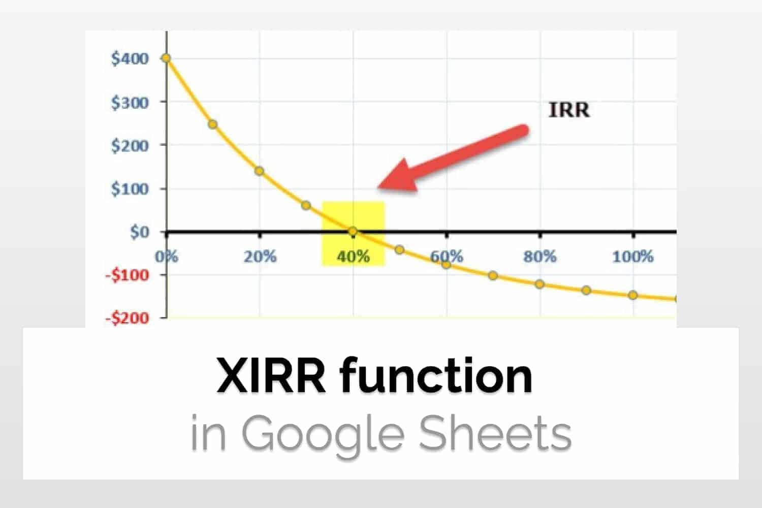
XIRR function is used to calculate the internal rate of return of an investment based on a specified series of potentially irregularly spaced cash flows. The internal rate of return is basically the annual growth rate based on some factors. These factors are namely, cashflow amount and cashflow dates.

In this table, you see the transaction amount for a business owner. Negative values represent the outflow of money and positive values represent the inflow of money into the business. The internal return rate is the value in percentage related to how many returns the business generated during this time. You can read more about the internal rate of return here. Also, note in this table that the transactions are not periodic, i.e. they don’t occur after a set amount of time.
IRR – Used if cash flows are periodic; XIRR – Used if cash flows can occur at any time
What is the difference between XIRR and IRR? In XIRR, the cash inflow and outflow can occur at any time, i.e. it is not necessary that your payments occur after a set amount of time. It is different from IRR in Google Sheets where it is calculated for periodic cash flow. Because of these reasons, XIRR is preferred over IRR.

We will see an example below to see in detail how to use it. But before that, let’s have a look at its syntax.
The syntax for XIRR function in Google Sheets
XIRR function in Google Sheets requires a table of cash inflow to run. The table should contain two columns, one for the date and one for the cash inflow on that date. The syntax for the XIRR function in Google Sheets is as follows.
=XIRR(cashflow_amounts, cashflow_dates, [rate_guess])cashflow_amounts: An array or a range of cells which contains the cash inflows(or outflows) related to the investment. It must contain at least one negative and one positive entry for the formula to work.
cashflow_dates: An array or range of cells which contains the dates on which the above transactions took place. This should be in Google Sheets recognised date formats. You can also check out the DATE() function for the same.
rate_guess: It is a guess of what you think XIRR would return. Google sheets needs a starting point to start their calculation and then arrive at the final answer. If you don’t have any idea about the same, you can omit it. It’s an optional attribute with the default value of 0.1.
The cashflow amount entries should be positive if the investment is returning a value, otherwise, it should be negative if you are investing money into the business.
Sample Usage
Let’s take the same example that we saw earlier in this article. There are two columns. One column contains the date and the other one contains the transaction amount.

Now the usage of the function is pretty straightforward. The first parameter would be the range A2:A7, since it contains the value of the transaction related to the business. The second argument is the references for the date. The value for the same would be B2:B7. We would keep the third parameter empty as we want to keep the internal rate at 10 percent. Hence the final formula becomes:
=XIRR(cashflow=XIRR(A2:A7, B2:B7)
Hence the XIRR comes out to be 0.34. Additionally, another way to do this is by inputting the actual array in the formula rather than giving the references for the cells. But obviously, the former method is much better than the latter one.
Conclusion
In this article, we read about XIRR and saw how to use the XIRR function in Google Sheets. We also read about the comparison between XIRR and IRR.
See Also
Want to know more formulas and functions in Google Sheets? Look at our definitive guide on Google Sheets which covers hundreds of such topics here. Enjoy reading!
Filter Data by Color in Google Sheets: In this article, we would have a look at how to Filter Data by Color in Google Sheets.
How To Calculate Standard Deviation In Google Sheets: We will learn how to calculate standard deviation in Google Sheets
Introduction to DATE function in Google Sheets: We will have a look at the DATE function in Google Sheets and see how to reference the month, day and year from another cell. We will also see how to change the date format in Google Sheets.