Syntax:=CUMIPMT(rate, number_of_periods, present_value, first_period, last_period, end_or_beginning)rate: The rate of interestnumber_of_periods: The total number of payment periods (number of installments)present_value: The value of the investment/borrowed amountfirst_period: The starting range of cumulative interest calculation (it’s always between 1 and last_period)last_period: The ending range of cumulative interest calculation (it’s always between the first period and Number_of_periods)end_or_beginning: Whether payments are due at the end (represented by 0) or at the beginning (represented by 1)
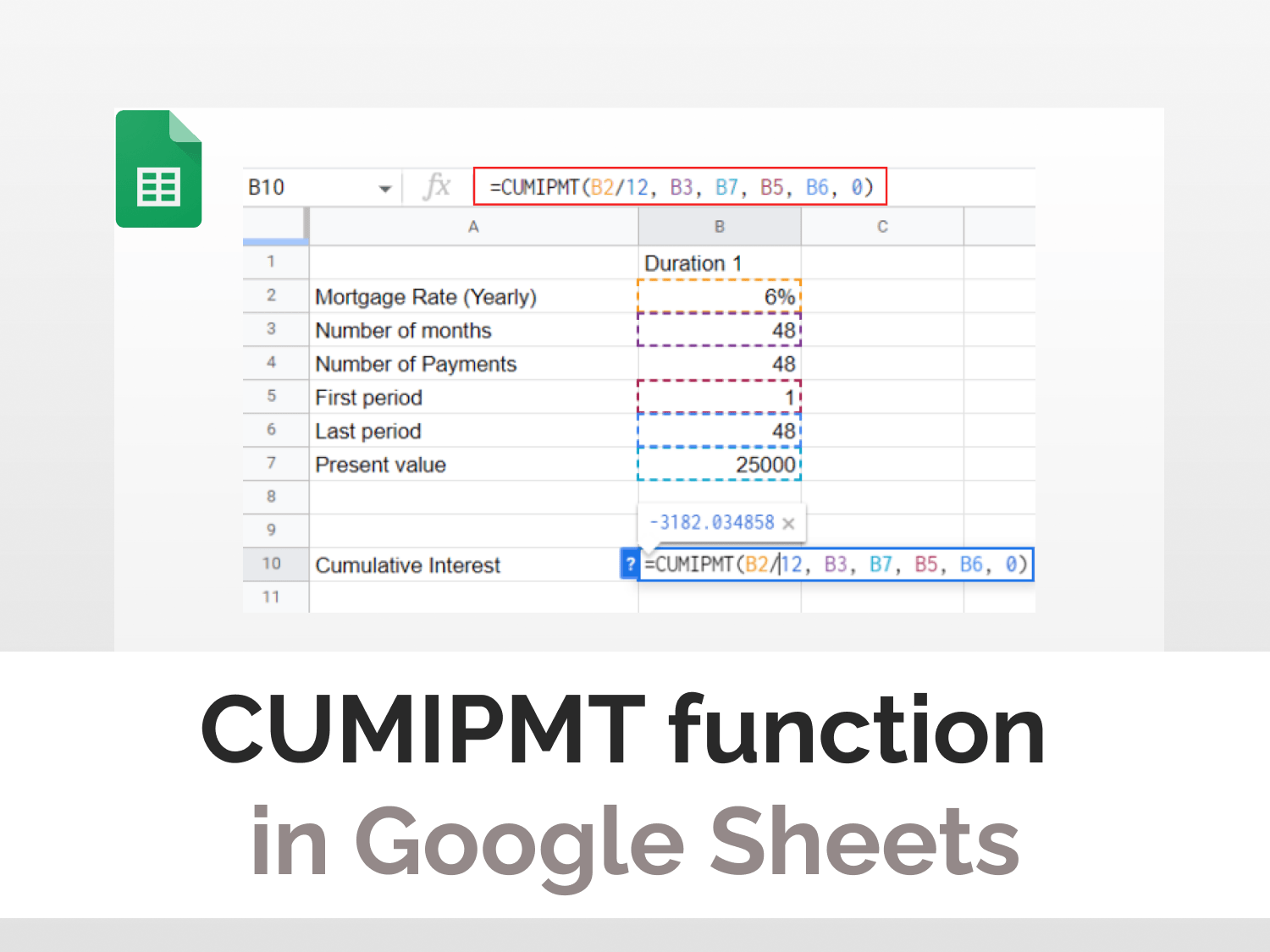
Sample usage:=CUMIPMT(6/12, 48, 25000, 1, 48, 0)
//It calculates cumulative interest for $25000 with an annual rate of interest at 6% for 48 monthly instalments
Sample Google Sheets template with formula here.
The CUMIPMT function in Google Sheets calculates the cumulative interest paid on a loan or investment (fixed principal) at a fixed rate of interest over a specified period.
The function is useful because it helps one calculate how much money will go towards paying interest. It can also be used to forecast the returns one can expect over time.
Utility of the CUMIMPT function
Let’s understand the utility of the CUMIPMT function in Google Sheets:
- You have borrowed a sum of money from a bank. What should be the ideal period to repay the borrowed amount?
- You plan to invest in a fixed deposit. How much should you invest to be able to buy a house 5yrs from now?
- You are being offered different loans at different interest rates and periods. Which one should you go for?
The CUMIPMT function in Google Sheets is an easy and simple way to answer questions similar to those above. It can help one plan their finances accordingly as it does all the complex financial calculations for you with a single click.
In this tutorial, our prime objective is to learn how to use the CUMIPMT function in Google Sheets. Let’s get our finances sorted by understanding the syntax of this function.
Understanding the CUMIPMT Function in Google Sheets
In the following example, we will discuss the use case of the CUMIPMT function in Google Sheets. We have a spreadsheet containing financial data about a loan. We will find out the cumulative interest to pay for different durations.
In the following example, We have a fixed rate of interest, number of months (duration), number of payments (frequency), starting period, end period, and amount. We have already calculated the cumulative interest amount for 48, 96, and 120 months respectively.
The different interest amounts for different periods help us choose the apt duration of our loan based on our current financial condition. The longer the duration the more interest amount one will end up paying.

How to implement the CUMIPMT function in Google Sheets
In this tutorial, we will start implementing the CUMIPMT function in Google Sheets.
The steps are as follows:
- Select the cell where you want to display the cumulative interest

- Begin your function with the ‘=’ sign. Type ‘CUMIPMT’. The google sheets will prompt this function, press enter key to autocomplete. The tooltip guide will appear along with the details.

- Enter the cell addresses for all the parameters and for the end_or_beginning parameter, and enter 0 if payments are due at the end or 1 if payments are due in the beginning.

Note: The mortgage rate has been divided by 12 to convert the interest rate monthly
The final formula, in this case, should look like this:
=CUMIPMT(B2/12, B3, B7, B5, B6, 0)

= -3182.034858 //this is the result the formula returns
The CUMIPMT function in Google Sheets tells us that for the period of 48 months, 6% annual rate of interest and $25,000 principle amount, one will end up paying $3183 as interest.
CONCLUSION
We have learned how to use the CUMIPMT function in Google Sheets using illustrative examples. Now, you are all set to start using this powerful statistical tool to your advantage.
The inbuilt CUMIPMT function in Google Sheets makes calculating cumulative interest a cakewalk. Using this powerful tool, one can easily make informed and data-driven decisions.
Frequently asked questions
What is the IPMT Function in Google Sheets?
The IPMT Function is categorized under Financial functions. The function calculates the interest portion based on a given loan payment and payment period. We can calculate, using IPMT, the interest amount of payment for the first period, last period, or any period in between.
How do you calculate the total interest paid over the life of the loan?
Total interest is the sum of all interest paid over the life of a loan or interest-bearing account, including compounded amounts on the unpaid accumulated interest. It can be derived using the formula [Total Loan Amount] = [Principle] + [Interest Paid] + [Interest on Unpaid Interest].
How do you calculate cumulative interest payments?
Compound interest is calculated by multiplying the initial principal amount by one plus the annual interest rate raised to the number of compound periods minus one. The total initial amount of the loan is then subtracted from the resulting value.
What is the PMT function in Google Sheets?
The Google Sheets PMT function is a financial function that calculates the payment for a loan based on a constant interest rate, the number of periods and the loan amount. “PMT” stands for “payment“, hence the function’s name.
See Also
Are you interested in learning more about how much you can succeed with Google Sheets? With so many powerful features of Google Sheets, you save time and effort.
We have several tutorials that cover tricks and tips in Google Sheets. You can discover them here.
Here are some articles you might be interested in:
https://blog.tryamigo.com/calculate-compound-interest-in-google-sheets/
https://blog.tryamigo.com/correl-function-in-google-sheets/
https://blog.tryamigo.com/import-yahoo-finance-data-into-google-sheets/