Create a Burndown Chart in Google Sheets-4 Min Easy Guide

Reading Time: 5 minutes

Table of Contents

What is a Burndown Chart in Google Sheets?

A burndown chart is a graphical representation of the work and time remaining for a project’s completion. A burndown chart in Google Sheets is used as a project management tool to track what task has been completed, what remains to be completed, and how much time remains for a project.

Why use a Burndown Chart in Google Sheets

A burndown chart in Google Sheets is handy for tracking the progress of a team’s work compared to what was originally estimated. It informs the team early on whether a project is on track and whether it will be completed on time.

Let’s say we have a set of 10 tasks planned for the week. We have set deadlines for all of the tasks. We want to track the actual completion date against the scheduled completion date. We can visualise this using a Burndown Chart in Google Sheets. We can also see how much more effort we need to put in if we lag behind the due date.

How to create a Burndown Chart in Google Sheets

Below is a step-by-step guide on how to create a burndown chart in Google Sheets.

Step 1: Create a Time Vs Planned Task

Create a column for the tasks completion date
Create a column of how many projects(planned) are left against a particular date.
Create a column of how many projects(completed) are left against a specific date.

Figure 1: Dataset of interest

Here, the first column is for the date on which the project is to be completed.
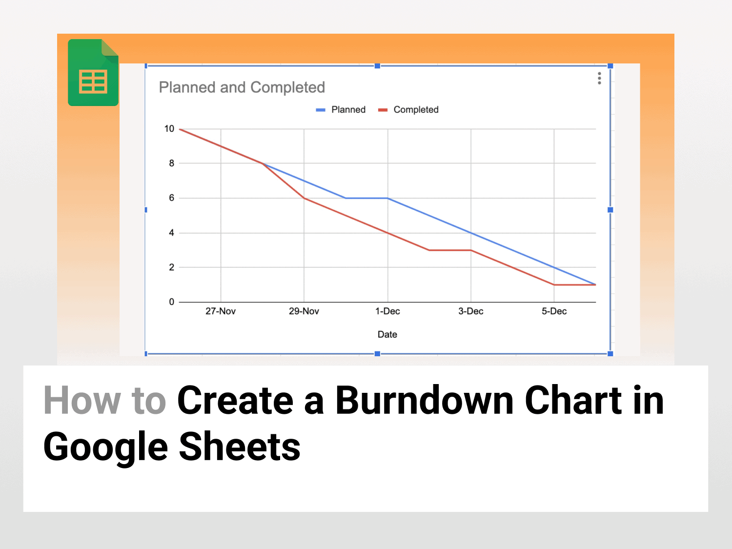
The second column is for how many tasks are left at a particular time. So, on the 26th of November, ten tasks are planned to be completed. Eight tasks are left on the 28th of November, i.e. two tasks are planned to be completed. Similarly, four tasks are left on the 3rd of December, i.e. six tasks are planned to be completed.
The third column is for how many tasks are left after completing some tasks. So, on the 27th of November, nine tasks were left to be completed, which means 1 task was finished. On the 29th of November, six tasks are left to be completed, i.e. four tasks have been actually completed.

Step 2: Insert Chart

Select the entire dataset by Ctrl + A (Windows) or Cmd + A (Mac).
Go to Insert → Chart.

Figure 2: Insert Chart

Step 3: Change Chart type to Line Graph

You will see that automatically a combo chart is inserted, which looks like this:

Figure 3: Auto-generated chart

Go to Chart Type and click the drop-down menu.
Select the Line Graph with pointed vertices, as shown below:

Figure 4: Select Line Graph

Congratulations, you have successfully created a Burndown Graph in Google Sheets.

Figure 5: Example of Burndown Chart in Google Sheets

Make a Copy of the Spreadsheet

How to create a Dynamic Burndown Chart in Google Sheets

Let’s suppose we want to create a dynamic burndown chart in Google Sheets, i.e. we want to automatically update the Completed tasks column on a daily basis to help us keep track of our projects and help us finish them within the deadline.