Objective – To understand various use cases of QUERY function with IMPORTRANGE in Google Sheets and how their combination can be used to achieve wonderful results.
Syntax=QUERY (IMPORTRANGE(spreadsheet_url, range_string), query, [headers])spreadsheet_url – It refers to the URL of the spreadsheet we want to retrieve data fromrange_string – It refers to the particular table/range in the spreadsheet
Example usage=QUERY(IMPORTRANGE(A1,"ALL ARTICLES!F6:N25"),"Select Col1")
//Retrieves column 1 from the sheet ALL ARTICLES
Sample Google Sheets template with formula here.
- Overview
- Why use the QUERY function with IMPORTRANGE
- How to use the QUERY function with IMPORTRANGE
- #1: Retrieve data from an external spreadsheet
- #2: Retrieve a specific column from an external sheet
- #3: Retrieve a list of items
- #4: Retrieve and sort items in descending or ascending order
- #5: Return the maximum value by department
- #6: Total salary by gender
Overview
Google Sheets QUERY and IMPORTRANGE functions are two of the most flexible and powerful functions on the platform.
The QUERY function is useful for its flexibility and ability to tackle a wide range of problems. It is similar to SQL query and makes database-oriented operations a breeze in Google Sheets.
On the other hand, the IMPORTRANGE function has one primary utility—to retrieve data from an entirely different spreadsheet.
While that is an amazing function to use, it is a bit limited in terms of what you can do with the data you import. But it can be made a great deal more useful by combining the QUERY function with IMPORTRANGE.
Why use the QUERY function with IMPORTRANGE in Google Sheets?
As you must have already guessed, they both have their limitations. The QUERY function with all its flexibility can only be useful in one sheet. On the other hand, the IMPORTRANGE function, while being an excellent long-range formula, is limited in terms of manipulating data.
Therefore, combining QUERY with IMPORTRANGE strategically mitigates these limitations. QUERY function offers its amazing query properties and IMPORTRANGE takes that into data located in other sheets. Great teamwork!
Combining the QUERY function and IMPORTRANGE: How it works
We will combine the IMPORTRANGE and Google Sheets QUERY functions by passing the entire IMPORTRANGE function as a parameter in the QUERY function. The QUERY-IMPORTRANGE combination will provide us with flexibility and range. Pretty awesome. Now let’s get to see how we can use the QUERY and IMPORTRANGE functions together.
Just to recap, the QUERY function has the syntax below:
=QUERY(data, query, [headers])- The first parameter is the dataset(usually a table in a spreadsheet)
- Query refers to the data operation we want to perform
- The final parameter is an optional header
Therefore, when we combine the QUERY function with IMPORTRANGE as above, the IMPORTRANGE function replaces the dataset parameter in the query function. The IMPORTRANGE function still does all it is designed to do. And the QUERY function becomes more sophisticated by relying on a dynamic dataset that it can utilize for its operations.
Note: IMPORTRANGE updates changes in the new spreadsheet when the source of its data is modified. This is handy because having to manually update changes in our spreadsheet can quickly become tedious.
How to use the QUERY function with IMPORTRANGE in Google Sheets
Now, let us with the aid of examples examine multiple ways to utilize this powerful combination of the QUERY and IMPORTRANGE functions in Google Sheets.
Example 1: Retrieve data from an external spreadsheet using the QUERY function with IMPORTRANGE in Google Sheets
In this example, we will learn how to retrieve data from a different spreadsheet using the IMPORTRANGE in the QUERY function.
Step 1: Set up the data
We are going to use the data from a recent article. The dataset is a table containing the recently published articles on our blog, as well as other information such as the author, the title of the article, the date created, etc.
Here’s the spreadsheet containing the data used in this article. Make your own copy of it to use in the examples.
Step 2: Enter the function and the parameters
Copy the URL given above and head over to a brand new spreadsheet.
- In a cell of your preference, enter the QUERY function by typing =QUERY
- Select the QUERY function from the dialogue (you can press Enter or Tab to select the suggested function).
- Paste the URL as the first parameter of the QUERY function. For now, we won’t be doing any manipulation of data; we just want to retrieve the dataset.
- So, we will set the query parameter of the QUERY function to Select* which means select all.
The complete syntax of the QUERY function with IMPORTRANGE in Google Sheets is given below.
=QUERY(IMPORTRANGE("https://docs.google.com/spreadsheets/d/1AA2JE6bi10V4ps17JrYzzHcluRbNZNwDhfOc_7mZHi8/edit","ALL ARTICLES!F6:N25"),"Select *")- Enter the complete formula and press Enter and fetch the data.

The table corresponds with what we have in the original spreadsheet. And thanks to IMPORTRANGE, any updates or changes on the original table will result in a corresponding change in the new sheet.
Now, if retrieving every column in a spreadsheet was the only thing we wanted to do, there wouldn’t be a need to go as far as combining two formulas. The IMPORTRANGE function can take care of that.
The usefulness of the QUERY and IMPORTRANGE combination lies in utilizing the best each function has to offer. So let us look at more examples.
Example 2: Retrieve a specific column from an external spreadsheet using the QUERY function with IMPORTRANGE in Google Sheets
Using the QUERY function with IMPORTRANGE in Google Sheets we can retrieve a particular column in a different spreadsheet. We will do this using the Select command.
Assuming we want to only see the articles in the previous table we retrieved, we can do this using the below command:
=QUERY(IMPORTRANGE(A1,"ALL ARTICLES!F6:N25"),"Select Col1")Here, “ALL ARTICLES” is the name of the spreadsheet, the exclamatory mark indicates that we’re referencing another spreadsheet, and F6:N25 is the range of the data. And “Col1” stands for the first column–which is what we want to retrieve.
On pressing Enter, we’ll get the data as shown below.

The QUERY function with IMPORTRANGE returned the articles column from the external sheet successfully.
Tip: instead of putting the long URL into the function every time, you can just store it in a cell, say A5. Then you can reference it in the formula.
Example 3: Retrieve the list of authors in order of most published articles using the QUERY function with IMPORTRANGE in Google Sheets
If we want to find out how many articles each author has published and to return a list showing that information in order of most published. We can do that using a combination of commands.
The formula for which is:
=QUERY(IMPORTRANGE(A1,"ALL ARTICLES!F6:N25"),"Select Col2, Count(Col2) GROUP BY Col2 Order by Count(Col2) desc")Let us deconstruct this formula. The IMPORTRANGE function retrieves the data from the URL in cell A1; the QUERY function, from the data imported by the IMPORTRANGE function, selects the data in column 2, counts the items in column 2, classifies the items in column 2, and arranges these grouped items in descending order, ie, largest to the smallest.
This may seem a little complicated but if you study the formula carefully or use the QUERY function more regularly, it should become less knotty.

To illustrate the next set of applications for QUERY with IMPORTRANGE in Google Sheets we will be making use of the employee data of a certain imaginary company. The table contains information about the various employees which includes their names, department, age, salary gender, and finally ethnicity.

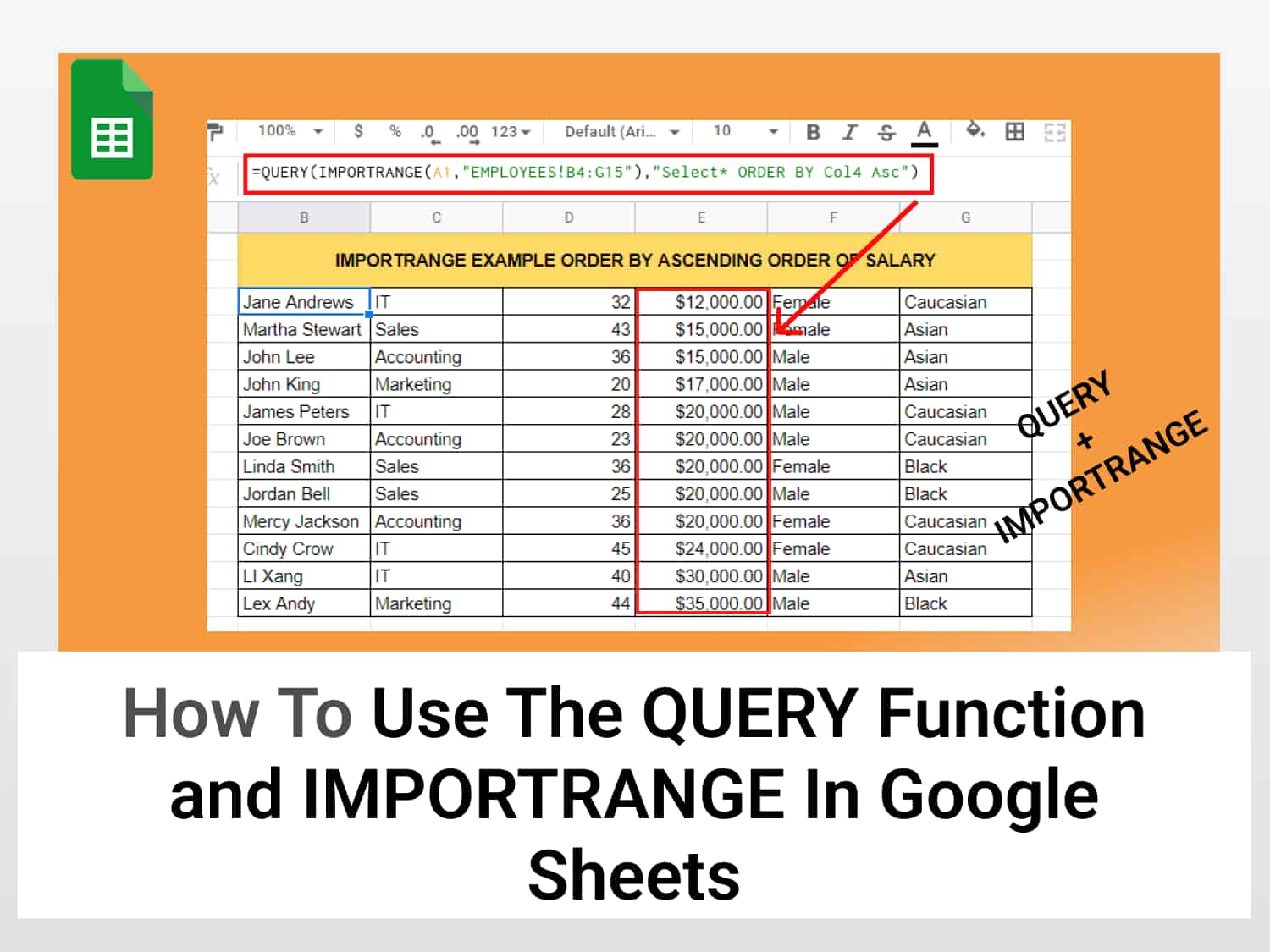
Example 4: Sort data in descending or ascending order
Let’s consider an instance where we want the QUERY with IMPORTRANGE to return data which are sorted in descending order of salary, i.e from the highest earner to the lowest.
This can be helpful to an organization that wants to review its salary structure.
For descending order, enter the following command.
=QUERY(IMPORTRANGE(A1,"EMPLOYEES!B4:G15"),"Select* ORDER BY Col4 Desc")
On the other hand, if we need to return the data in ascending order of salary i.e from the least to the highest, use the Asc command in place of Desc.

Example 5: Return the highest values by department using the QUERY function and IMPORTRANGE in Google Sheets
If the company wants to see the highest salary levels in the various departments, it can do this using a combination of MAX and GROUP BY.
The IMPORTRANGE function will retrieve the data from the original table in another spreadsheet. And the QUERY function will perform operations on it using MAX and GROUP BY.
We are going to see how.
Enter the formula below in a cell.
=QUERY(IMPORTRANGE(A1,"EMPLOYEES!B4:G15"),"Select Col2, MAX(Col4) group by Col2")
The right column shows the maximum salary corresponding to the various departments in the left column.
Example 6: Total salary by gender
We could also be interested in seeing how much a gender earns in the company.
We will be using SUM to aggregate the salary then use CONTAINS to indicate that we are interested in retrieving the salary for the female employees.
The QUERY formula with IMPORTRANGE to return the total salary of female employees is as under.
=QUERY(IMPORTRANGE(A1,"EMPLOYEES!B4:G15"),"Select sum (Col4) Where (Col5) contains 'Female'")
The table above shows the total amount earned by the female employees.
There are so many ways to combine the QUERY function with IMPORTRANGE in Google Sheets and achieve different results. Also, note that all our operation so far has been on data in another spreadsheet. That is why combining the query function with IMPORTRANGE is very effective.
Conclusion
The QUERY function can be combined with IMPORTRANGE to achieve amazing results. Because while the QUERY function isn’t designed to operate outside a spreadsheet, the IMPORTRANGE does this primarily. And thus together, the QUERY and IMPORTRANGE functions work together to perform wonderful functions.
See also
If you enjoyed reading this then you might want to check out similar articles and general Google Sheets tips on our blog:
Reference data from other sheets in Google Sheets
VLOOKUP from another sheet in Google Sheets
Easy Way To Scrape Google Search Results And Auto-update The Data