How To Use The DSUM Function In Google Sheets

What it does – calculates the sum from a well-structured data using an SQL-like query.

The DSUM is a database sum function, the ‘D’ in the name DSUM stands for Database. This function requires a structured table whereas other similar functions like SUMIF and SUMIFS don’t require a structured table.

The DSUM function in Google Sheets is a powerful tool that can be used to sum up entities based on a given set of conditions (also known as criteria).

The DSUM function can be used to make inferences about the performance of employees or the product manufactured and a wide range of other calculations based on a database table.

• Using the DSUM function – Method One
• Using the DSUM function – Method Two
• Using the DSUM function with wildcards
• Calculate the sum from a database
• Some things to note

How to use the DSUM Function in Google Sheets

Step 1: Gather Data

In order to use the DSUM function in Google Sheets, we first need to specify the database using appropriate headings. Let’s assume that after investigation, Apple came up with the following data with regard to the sale of its different categories of products in each quarter:

Note: All cells containing numbers in the article have been formatted to include arrows and zero decimal places. You can do the same by selecting the data and navigating to Format→Number→Number.

Step 2: Specify the criteria

Let’s assume that a manager at Apple wants to find the total number of phones sold in the first two quarters from the data generated.

To specify the criteria we navigate to a new cell and manually input it as column labels followed by the given conditions as shown below:

Note: The column labels should be verbatim to the ones used in the database.

Step 3: Calculate the result

Next, we input the formula specified below into a new cell to find the required total:

=DSUM(A1:C17, "Number of Units sold", F6:G8)

In this example we were supposed to add only two values, thus we could have manually found the total as well. However, when faced with large data sets, computing the aggregate of particular data values becomes impossible. For such problems, the DSUM function in Google Sheets can be a real lifesaver.

Alternative methods:

1. Instead of specifying the two quarters in our example, we could have also just inputted “<3” in cell F7 to denote the first and second quarters.

2. Instead of specifying the field as “Number of Units sold”, the formula would have worked even if we had used the number 3 (to denote the field as the third column of the database).

3. Instead of, specifying the cell range of the criteria, one can also manually input it  into the formula:
   =DSUM(A1:C17, 3, {{“Quarter”; “<3”}, {“Product”;”Phones”}})

In our example, we tried to find the sum of the number of units sold for those products that satisfied both the two conditions. Let’s have a look at a few other examples to understand the different types of criteria input that DSUM allows for.

Different ways to use DSUM Function in Google Sheets

The DSUM function can work with all logical conditions that one might use in an IF statement while using Google Sheets. Thus, DSUM can work with <,>,<=,>=, and wildcard characters as well.

Using the wildcard characters 

Wildcard characters are a diverse set of characters which can be used to select a group of similar strings at a time. These characters can be used in the range of cells containing the user-specified criteria when using the DSUM function.

For example, if we had the following data, and we needed to find the total units sold by all salesmen whose name starts with ‘P’ in quarters 2,3, and 4, we could use the DSUM function to find the sum as shown below:

The above-mentioned picture uses the asterisk (*) wildcard that is used to represent or take the place of any number of characters. In the above situation, we use DSUM to calculate the total number of units sold by all salesmen whose names begin with the letter ‘P’ (denoted by the asterisk) in quarters 2,3, and 4.

Similarly one can use other wildcard characters such as ‘?’ (Represents one character in a string). For example, “T?m” will represent “Tom”, “Tim”, “Tam” and so on), and ‘~’ (tells the software that the next character should not be considered a wildcard).

Refer to the image below to notice that when we input “T?m” as the criteria under salesmen we are summing up the number of units sold by all those salesmen whose name starts with ‘T’ and ends with ‘m’ with only one character in the middle. Simultaneously, when we input “T~*” we only add the number of units by the salesman whose name is “T*”. 

How to use the DSUM function in Google Sheets to calculate the sum from a database

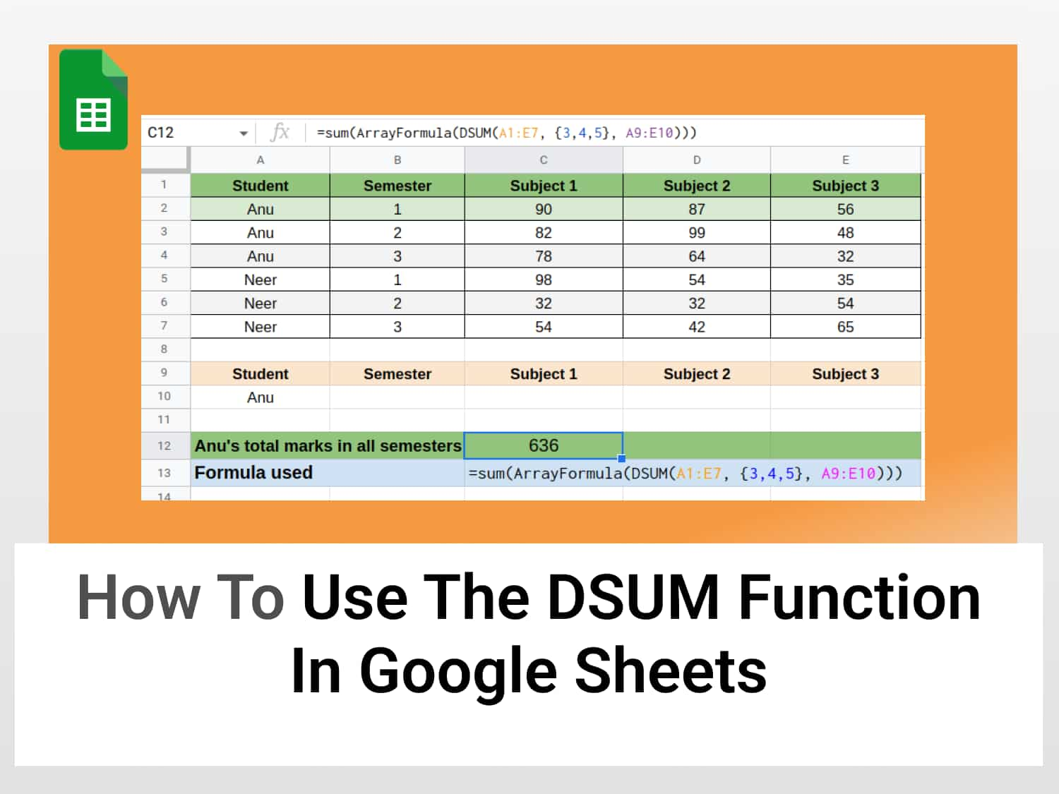
Lets’s say, we have a database of a class with information about some students as follows.

Our objective is to find the total marks scored by Student A in all the semesters. In this situation, we need to sum up the marks from multiple columns. The DSUM function in Google Sheets lets us easily achieve this.

As we have to perform DSUM for multiple columns. We need to sum it up. Therefore, we sum up the array of sums received by applying DSM.

The syntax should be like this:

=sum(
     ArrayFormula(
        DSUM(database, {field 1,field 2,field 3,...}, criteria)
     )
)

Follow the stem given below on how to use the DSUM function in Google Sheets to calculate the sum of data arranged in an array.

• Select the cell and start typing =DSUM. Google Sheets will start prompting the DSUM function, press Enter or Tab to autocomplete.
•  Add the database range in the first parameter. In this case, it will be A1:E7.
• Now, for the field section add the indexes of subject1, subject2, and subject3 inside curly braces. It should look like this:
  
  =sum(ArrayFormula(DSUM(A1:E7, {3,4,5}, A9:E10)))

• As we want to calculate the sum of marks for all subjects in all the semesters, we will type the name of the student as the condition and leave the rest of the cells empty. It should look like this:

• The final output looks like this. 

This is how we use the DSUM function in Google Sheets to calculate the marks of students in all subjects for all semesters.

Important things to remember

1. The criteria range can be located anywhere on the sheet. However, it is a common practice to mention the criteria range below the dataset.

2. In case, more conditions need to be added, the formula will have to be edited to include the new conditions as well.

3. DSUM should only be used to add data when the columns are contiguous. In case the columns are not contiguous normal SUMIF function may be used.

4. In case, there are no numeric values in the mentioned “field”, the DSUM function will return 0 as its output.

Conclusion

DSUM can be a very convenient and effortless function to use when you have a well-structured database, with specified column labels, and specific conditions. Once the inputs are determined, one can simply insert them into the function to get the desired result.

FREQUENTLY ASKED QUESTIONS

What is the difference between DSUM and SUMIF?

DSUM requires column headers for both the range and criteria whereas SUMIFS doesn’t require column headers. That is why Google Sheets uses the term database in connection with DSUM as database means that column headers should exist.

Why is the DSUM function not working?

The reason for the DSUM not working could be several. Some of the most common ones are incorrect criteria, missing headers, missing data in a named range, and referencing a column label to retrieve data from a database table in a pivot table. For simpler calculations, the SUM or the SUMIF function may be used instead.

See also

Google Sheets can be a very powerful tool only if you know how to. Learn about the other tools that Google Sheets offers through the articles below

https://blog.tryamigo.com/sumifs-function-in-google-sheets-quick-guide/

https://blog.tryamigo.com/sumproduct-function-in-google-sheets/

https://blog.tryamigo.com/arrayformula-in-google-sheets/