What it does- Calculates the work date that is the indicated number of working days before or after a date.
Syntax
=WORKDAY(start_date, num_days, [holidays])
start_date – the date from which to begin counting
num_days – the number of working days before or after the start_date. A positive value counts forward from the start_date while a negative value counts backwards.
holidays – optional; excludes dates in this list, entered either as a range of dates or an array of numbers
Sample Usage=WORKDAY(“25/09/2022”,12,“A2:A5”)
//This will return the date 12 workdays away from 25th Sept, and exclude dates mentioned in A2:A5.
Note
Only workdays Mon-Fri are included.
Sample Google Sheets template with formula here.
We can use the WORKDAY formula in Google Sheets to calculate the invoice due dates, expected delivery times, the number of days of work performed, and project completion dates taking into account only the working days.
The WORKDAY function in Google Sheets is a useful tool and we are going to learn some of the useful things we can do with it with examples.
Overview:
- Calculate the project completion date
- Exclude holidays from workdays
- Project start date based on delivery date
- Get all workdays
- Custom workdays and weekends
How to use the WORKDAY function in Google Sheets
In this section of the tutorial, we’re going to learn the different ways we can use the WORKDAY function in Google Sheets for a variety of purposes.
Let’s begin with a simple example.
Calculate the project completion date using the WORKDAY function in Google Sheets
Suppose we have a project beginning on September 25, 2022 which will take 10 days to complete. We can use the WORKDAY function in Google Sheets to compute the days on which it’s expected to be completed after excluding the weekend.
The formula will be as shown below.
=WORKDAY(DATE(2022,09,25), 10)Note: We need to embed the DATE function within the WORKDAY function or enclosed the date under quotation marks as otherwise the function will not recognise the date and will return an error.
This will return the date as Friday, October 7, 2022.

We can omit the DATE function by enclosing the date by a pair of quotes.

Another method is to reference cells that contain the start date and the number of days.
For the above example, the formula will be as follows:
=WORKDAY(A3,B3)Where A3 is the cell reference for the start_date and B3 contains the value of the number of days.

If there are multiple projects with different starting dates and the expected number of days required, we can calculate the end dates by using the same WORKDAY function. All we need to do is to enter the start dates and the number of days in the corresponding cells underneath and drag the formula to return the results for all the projects.

Using the WORKDAY function in Google Sheets to calculate project completion dates excluding holidays
The above examples did not consider the other non-working days besides the weekends and so the completion dates returned could be earlier than they’d actually take.
We can rectify this by specifying the holidays in that time period.
Let us consider it with an example.
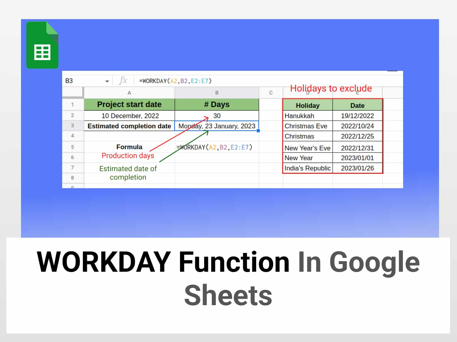
Let us assume that a project is to be completed in 30 days and is scheduled to start on 10 December 2022.
What we need to do is list the holidays in a separate column and reference the range of the cells as shown below.

In order to calculate the estimated completion date of the project taking into account the holidays and the weekends, we can use the formula shown below.
=WORKDAY(A2, B2, E2:E7)Where A2 and B2 are the cells that contain the start date and the number of days respectively, and E2:E7 is the range of cells with the holidays.
Upon entering the formula, we get the following result: Monday, 23 January, 2023.

Calculating the start date of a project based on the delivery date using the WORKDAY function
We can use the WORKDAY function in Google Sheets to determine the date on which a project should be begun considering the date on which the project has to be completed and the estimated number of days it’d take to complete.
Suppose that we have a project which would take about 20 days to complete and is to be completed by 20 December 2022.
The formula will be as given below.
=WORKDAY(B1,B2)Since we’re counting backwards from the project deadline, we use a negative number for the number of days.
Upon entering the formula, we’ll get the result as shown below.

Using the WORKDAY function in Google Sheets to fetch all the working days
We can use the WORKDAY function in Google Sheets to generate all the working days in a given period.
Enter the first day of the month in a cell (in this case, A1). Then under that cell, enter the following formula:
=WORKDAY(A1, 1)The nun_days argument is 1 since we want to get all the working days–the project completion day being essentially 1.
Enter the formula and drag the formula cell till the days of the month is exhausted.

As we can see from the screenshot, only the working days are returned with the weekends omitted.
Throughout this tutorial, we have only considered the examples assuming that our working days are from Monday through Friday. But what about cases where Saturday is a working day and the weekend is not Saturday and Sunday?
Fortunately, there is another function called the WORKDAY.INTL. We can use this function to customise the weekend and the number of days off in a week. Let us learn about it.
How to use the WORKDAY.INTL function in Google Sheets
Let us assume that the working days at a company are from Monday through Saturday so that there is only one day weekend instead of the usual two. In this case, we need to use the WORKDAY.INTL function instead of the WORKDAY function which assumes Saturday and Sunday as weekends.
Syntax of the WORKDAY.INTL function in Google Sheets
=WORKDAY.INTL(start_date, num_days, [weekend], [holidays])The weekend argument is an optional parameter and defaults to 1 if not specified. 1 is for Saturday and Sunday as weekends. The rest of the arguments is the same as for the WORKDAY function.
Let us consider an example.
Suppose we have to complete a project which would require 30 working days scheduled to begin on October 3.

To calculate the estimated date of completion of the project using the WORKDAY.INTL function in Google Sheets, we can use the following formula.
=WORKDAY.INTL(B1,B2,11)Here B1 is the cell that contains the start date and B2 the number of days. We use 11 for the weekend argument as that is the code for Sunday being the only weekend.
For more information on the WORKDAY.INTL function in Google Sheets and the number codes for different weekends, visit this page.

There are a bunch of other things we can use the WORKDAY function in Google Sheets for (as also the WORKDAY.INTL function) but they are for another day.
Conclusion
The WORKDAY function in Google Sheets is a very handy tool and can be used for a variety of purposes, as we have learned. I hope this article has been helpful.
See also
Working with the WORKDAY function in Google Sheets is just one of the many things you can do with Google Sheets for. We have a number of tutorials that cover tricks and tips in Google Sheets. You can discover them here.
Here are some related articles you may be interested in:
https://blog.tryamigo.com/how-to-use-the-weekday-function-in-google-sheets/
https://blog.tryamigo.com/how-to-insert-current-date-in-google-sheets/
https://blog.tryamigo.com/how-to-add-a-date-picker-in-google-sheets/